This post was written as a cursory version of a future part in my open book, understanding blocckDAGs and GHOSTDAG
In the previous posts we analyzed blockchain fee markets and isolated some unsavory properties that manifest as their equilibria: race-to-the-bottom, starvation, and price aberration. We named these the three woes. In the current post, we do the parallel analysis for blockDAGs. In the next post, we discuss how these differences affect the manifestation of the tree woes, and conclude the discussion.
The current post is by far the most mathematically involved in the series. To make it welcoming to a less technical crowd, I delegated the computational work to clearly separate sections and did my best to ensure the post is consistent and self-contained if they are skipped.
This post double-serves both as a layman exposition and for recording new observations that I am currently inspecting. In particular, I add interesting computations and results to this post as I find them. These extra-hard sections, marked with a double star, can rely on arbitrarily advanced math (though currently, it doesn’t go beyond advanced undergrad), and are not written as “educational content”. They are mostly here so I could easily share them with colleagues.
Pure Fee Markets With Multiple Leaders
We now need to extend the mining game we defined for blockchains to accommodate several miners. For simplicity, we assume that there are blocks per round (in reality, the number of blocks per round fluctuates around an average that can change with the network conditions), where each block was created by a different miner, and that the miners do not cooperate in any way.
The offering rounds remain the same, but the payoff rounds change. Here, each miner indeed reports a choice of transactions. But if several miners include the same transaction, its fee will go to one of them uniformly randomly.
Remark: OK, it is not exactly uniformly randomly. What actually happens is that the miners themselves are randomly shuffled: they are numbered from to in some random way. If two miners include the same transaction, the one with the lower number gets it. In other words, we don’t resolve the conflict per transaction, but per block. If Alice and Bob both included the same two transactions, then either Alice or Bob will get the fee for both transactions. There is no scenario where Alice wins one fee, and Bob the other. However, if we consider only one of the transactions, it will go with probability half to either Alice or Bob (assuming there are no more miners). In formal terms: the probability that one transaction goes to Bob depends on the probabilities that other transactions go to Bob, but the marginal distribution of a single transaction is uniform across all miners who included it.
This dynamic kind of shakes the ground at the feet of the miners, which is a good thing because the entire point I’m trying to make is that Bitcoin miners are just a bit too comfortable. Note that the source of unease is not the randomness itself, miners, above all, are very used to randomness. What makes this setting truly interesting is that now the choices of one miner affect the profit of another miner. Bob’s expected value depends on Alice’s choices. It is the consequences of this phenomenon that we seek to understand.
Equilibria Analysis
Strictly speaking, we need to analyze the equilibria strategies for both users and miners. Like before, we can’t do a precise analysis of the users, and while approximate models are possible, we will be satisfied with a qualitative discussion. This discussion will start very similarly to the case for block chains, but will have wildly different outcomes.
But analyzing the miner now becomes much more demanding, compared to the trivial equilibrium we had for blockchains (which was “just take the most profitable transactions”).
At the payoff round, the state of the game is a list of fees, which we will denote . Say that each miner only has to select one transaction (that is, ). A strategy is specified by a list of probabilities , which we interpret as “include the transaction paying a fee of with probability ”. If is two, then we need to specify a probability for any pair of transactions, and so on. In fact, as long as is sufficiently smaller than , the number of possible choices grows exponentially with (the exact number is given by a binomial coefficient).
To avoid this complexity, we will first assume that each miner only chooses one transaction. That is, that . Computing the exact answer for higher values of is quite difficult, but we will see how it can be simply approximated very well.
Another bane of our existence is that, since there are miners, and the strategy of each miner has probabilities, then there are in total probabilities in their combined strategies. Maximizing for that many variables is still quite daunting.
Fortunately, we can leverage the symmetry of the problem. Since all miners have the exact same information and options available to them, we can assume that there exists a symmetric equilibrium, and in fact, it is the only stable equilibrium (though actually proving this requires some heavy machinery). This means that we only need to solve for variables, describing a single strategy that all miners use.
Even under these assumptions, solving the general case is still quite a headache. So instead, we will consider three much simpler yet very illuminating cases:
- Two miners selecting one out of two transactions (, , )
- Two miners selecting one transaction (, , general )
- Uniform general case (general , , and , but )
First Case
This is the simplest case that is not trivial. It contains enough complexity to exhibit the consequences of multiple leaders quite nicely.
Recall that we consider two minutes that select one out of two transactions. Let us denote the fees they are paying and , and assume that . We can describe a strategy by a single number , which we understand as the probability of including , whereby we include with probability .
What is the best strategy?
Before jumping into the calculus, let us try some natural candidates and see how they fare.
Strategy I - Maximum: Select . That is, .
This strategy ignores the existence of the other miner and follows the optimal strategy for the single miner case. What is its expected profit?
Recall that we consider the case where both miners apply the same strategy. Hence, both miners will select , and the probability for each miner to gain the fee is , resulting in an expected profit of .
For and , the expected profit is . What about and ? Well, the expected profit doesn’t really care about the actual value of , as long as it is lower than , so it remains .
Strategy II - Uniform: Select either or with the same probability. That is, .
The miners become aware of the fact that collisions harm their expected profit and try to avoid it by flipping a fair coin. What would be the expected profit here?
There are four cases, each happening with the same probability of :
- Both miners selected , expected profit is
- Both miners selected , expected profit is
- I chose and other miner chose , expected profit is
- I chose and other miner chose , expected profit is
Since all events are equally probable, the expectation is just their simple average.
For and this comes out , which is clearly worse than the maximal strategy. But for and , this comes out $74.625%, which is better!
So if neither of these strategies is optimal, what is? We will work out the answer using some high-school-level pre-calculus: we will write the expected outcome as a function of and derive it to find its maximum. I will defer the calculation itself to the next section (that you can skip if you don’t feel like doing math).
The upshot of the calculation is the following:
Strategy III - Optimal: select with probability
The expected profit from this strategy is
Let’s see how we did! First, for and we get a profit of which is ever so slightly higher than the maximal strategy. For and we get which is again just above the random strategy. The impressive feat is that it is better than both at the same time.
In hindsight, it should not come as a surprise that the maximal strategy is almost optimal first case: if one transaction is 100 times more profitable than the second, then surely this offsets the expected profit lost by a chance of collision. It should also come as no surprise that the uniform strategy is almost optimal for the second: if the transactions pay about the same, then choosing one over the other doesn’t meaningfully change the profit, so it is better to do whatever possible to reduce the chance of collisions.
What happens around the middle, say at and ? Here the maximal strategy still expects , but now the uniform strategy nets , while the optimal strategy gives .
We finally note that the optimal strategy doesn’t actually depend on the values and , just on the ratio between them. We can see this by rewriting the expression we got:
The optimal strategy is the same whether and , or whether and . Multiplying and by the same number doesn’t change the optimal strategy (though the expected profit of this strategy does get multiplied by ).
For that reason, we can just assume , and that , and plot the expected profit from the optimal, uniform, and maximal strategies as a function of :
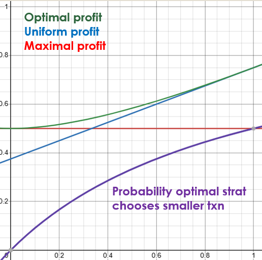
I also plotted the probability is chosen as a function of .
We see that the optimal strategy kind of morphs from the maximal strategy around to the uniform strategy around , which makes a lot of sense.
Remark: We can also compute that the shift in optimality between the uniform and maximal profit happens exactly when . For example, if and we easily see that the maximal and uniform strategy both have an expected profit of . The optimal strategy still beats both with .
The Computation*
One easy way to generalize the computations we did for the maximal and uniform strategies is to use a probability table. In such a table, each row represents a choice by one miner, and each column represents a choice by the second miner. The matching cell is the expected profit conditioned on these choices. The title of each row/column is the probability that the miner chose this option, so the probability of each cell is the product of the probabilities written in the title of its respective row and column. Sounds complicated? An example will make it much simpler.
For the maximum strategy, we have the following table:
So we see that the expectation obtained in the top-left corner has probability , and the rest have probability .
When we switch to a different strategy, we do not change the values in the cells. The expected profit given some particular selection by the miners remains the same. The only thing that happens is the probability that this selection will actually occur.
For the uniform strategy, we get the following table:
We see that here all cells have the same probability of , making the total probability just the sum of all cells divided by four. In other words, their average value.
In the general case, we have a probability to choose , so we obtain this table:
So now we follow the same procedure, we multiply each cell by the headers of its row and column, and sum the results:
and you can verify that this simplifies to
I will leave it to the reader to derive this expression with respect to , compare it to zero, and solve for . The final result is:
as expected.
Substituting this value of into the equation we found for the expectation gives the expression we got for the optimal expectation, as the reader is invited to verify.
Second Case
Now we have two miners () selecting one () out of transactions.
The solution, it turns out, is best expressed in terms of what’s called a harmonic average. It seems a bit weird at first, but it has a nice motivation.
The standard way to average numbers is called the arithmetic mean, defined for a list of numbers as
The harmonic mean is a different way to average numbers, that is more suitable to our computation. It is defined like this:
I wrote a beautiful segment about the harmonic mean and how you already know, but then I realized that it interrupted the entire flow of the post, so I deferred it to an optional section below. Suffice it to say, if we think of the everyday arithmetic mean as the correct way to average speeds, then the harmonic mean is the correct way to average rates.
As usual, I will defer the computation to a skippable section below.
The result is the following strategy:
Before we move on, we note that one can (quite easily) find for any values such that, according to the formula above, .
We call such instances degeneracies. We handle degeneracies in a later section, but for now, we will remain in the regime where no degeneracies happen, and this solution works.
The expected profit for each miner in this case is given by .
The Harmonic Mean and How You Already Know It
The harmonic mean might seem a bit… alien, but you’ve actually used it before without even realizing it. When you were a kid, you were probably given an exercise like this: if one builder builds one wall in three days, and another builder builds one wall in two days, how long would it take both builders to build two walls together?
We can’t just add the days up, that makes no sense. To correctly compute the answer, we realize that if a builder builds a wall in days, then they build walls in a day. The second builder builds walls in a day, so together they build walls in a day. We translate this quantity back from “walls per day” to “days per wall” by taking the reciprocal again. This gives us how long it would take to build one wall, so we multiply it by two to get:
The key insight is that the arithmetic mean is the correct way to average speed, while the harmonic mean is the correct way to average rates. To hit the nail on the head, you can convince yourself that
The Computation**
Say that there are two miners selecting one of the transactions paying . Given a strategy . Say the first miner selected , conditioned on that, their expected profit becomes . Since they choose with probability , their expected profit from this transaction alone is obtained by multiplying throughout by , getting .
To make things a bit simpler (and more readily generalizable) we can define the function and obtain that the expected profit from alone is exactly .
Hence, the total profit is given by the function:
We want to maximize this function with respect to the constraint (we will ignore the constraints for now).
By using the method of Lagrange multipliers, we can find that there is some real such that for each we get the equation
but since the only part of that depends on is the summand these conditions can be rewritten as
One can verify that after differentiating and isolating we find the relation which we plug into the constraint to obtain which after some rearrangement becomes as needed.
By plugging this optimal strategy into we obtain the maximal expected profit.
Third Case
The general case is a bit involved but becomes much simpler if we assume all transactions pay the same fee . In this case, the problem becomes much more symmetric and it is easy to conclude that the uniform strategy is the equilibrium (to prove that one can e.g. use the observation that an equilibrium strategy for transaction selection must be symmetric, and show that non-uniform strategies provide lower expected profit).
We can ask ourselves, if we add a new transaction, how high would it have to be to be non-degenerate? It is easiest to express the value of the transaction as and see how low could be without hitting degeneracy. Say we have transactions of value and we add a single transaction of value . Then for the transaction to have positive inclusion probability it must satisfy
I will leave the computation to you, but it comes out .
This doesn’t look very good, does it? Even if there is a decently small queue of transactions, we get that to be included one must have .
Well, we should not be disappointed by seeing only a slight improvement, because two leaders are only slightly better than one. What happens when there are many?
I didn’t explicitly write down the degeneracy formula for miners selecting one out of transactions, but there is one. If we plug transactions of value and a single transaction of value into this formula, we get that the transaction has positive probability if
This is already much better! It might not seem like much, since there are typically a lot more transactions (which could be in the thousands) compared with leaders per block (which are, at best, in the low dozens). However, the thing is that this expression decreases exponentially with while being only linearly close to .
For example, if we consider again the case of and now increase the number of leaders from to we see that significantly reduced from 99% to… 91.4%. Wait… that’s still not very good either, is it? Of course, because we are only limiting ourselves to one transaction per block! In fact, if and we are essentially considering a situation where the network is congested ten times over!
Now, increasing is where things get really complicated, even for two miners and uniform transactions. What causes the complication is the dependence between events. Since a miner can include both the second and seventh transactions, we have to take into account all possible overlaps with all other miners which creates a terrible mess. However, one can prove that even through that mess if all transactions pay a fee of , a transaction with fee has positive inclusion chances if
This is looking much better. We can now compute the degeneracy not as a function of the absolute number of transactions, but their fraction of the total capacity. That is, we consider uniform transactions, If we get that the network is exactly in full capacity. If we get that we are at half capacity, etc.
One can use the formula above to prove that if , the bound on is approximately . What does this mean?
If the network is exactly fully congested, that is , we get a threshold of about which is already a noticeable improvement, but that’s just the worst case! If the network is only half congested, that is, , this becomes ! Even when the network is at twice the full capacity we get that the threshold . Heck, even at ten times the throughput, we get the bound Compare this to Bitcoin, where once congestion hits, we are at a round .
General Case For Selecting One Transaction**
For completeness, I will provide the computation for a general number of miners sampling one out of a general number of transactions paying arbitrary fees .
For technical reasons, it will actually be more comfortable to talk about miners. This will allow us to assume the point of view of one miner, and write their profit in terms of what the other miners do.
The computation starts similarly. We ask ourselves, for the strategy , what is the expected profit from specifically for a particular miner.
First of all, the probability that the miner even selects is . If none of the other miners selected , which happens with probability , then the profit is . If exactly one miner also chose , then the expected profit is . For each given miner, the probability that this miner selected while the rest selected something else is . Since there are ways to choose one of the miners, we get that the total probability of the event “exactly one other miner selected ” is . We can extend this logic and say that the probability that exactly different miner selected is given by and in this case the expected profit is .
We can encode all this into the function and get that the expected profit for the strategy is given by
If we try to proceed in the computation as is, we will run into notational inferno. Instead, we first try to find a nicer expression for . This is a bit delicate:
The upshot is that is the unique solution to the separable differential equation with respect to the boundary condition (where uniqueness follows trivially by Picard’s theorem).
Solving this equation is direct, so I will leave it to the reader, but it follows that the solution corresponding to these boundary conditions is
Hence, the function we want to maximize is: and we do it again by using Lagrange multipliers.
I will spare you the details, but tell you the result. First, we introduce the power mean: (You are welcome to check that and are the arithmetic and harmonic means respectively.)
By doing a computation very similar to the one we did for two miners, we find that the optimal strategy is given by but to make this formula just a bit easier on the eyes, we return to the assumption that the total number of miners is and obtain the solution . The expected profit is then given by
and the non-degeneracy condition is
Degeneracy Reexamined**
Consider a situation where there are transactions with a fee and an th transaction with a fee . Clearly if then there are no degeneracies, how low/high can be without creating degeneracies? We know that no degeneracies exist for the case so we will assume there are at least three transactions in total.
One can easily compute that in this case, we have so the non-degeneracy conditions become
Note that we only need to verify this holds for and , as we assumed all fees are one of these two. One can check that the non-degeneracy condition we get by substituting always holds. This tells us that can be as high as we want without creating a degeneracy. This is already surprising: if there are at least two transactions, and they are all paying the same fee, then adding one new transaction, no matter how astronomic it fee might be, cannot make the other transactions degenerate. There is always motivation to leave some probability for the lower paying transactions. This is not true if we add more than one transaction though. Actually, it is not hard to show that if there are transactions of value , we obtain the condition
The non-degeneracy condition we get for is easily shown to be
Again, we shift our perspective a bit to assume that there are transactions with fee , to which an additional, th transaction with fee was added, to obtain that the condition for the newly added transaction to be non-degenerate is simply
This is already much better than the single leader (single transaction case), where if it instantly becomes degenerate, whereas if then it instantly renders all other transactions degenerate. However, the lower bound seems to approach pretty fast. If , then we get that is only allowed to be smaller than the average by a tiny amount.
But here’s the thing: in the case, assuming is the same as assuming that the network is extremely congested. Obviously, if there are a million times more transactions paying a fee of than the network can contain, there is no reason to acknowledge any transaction paying a fee of . To get a true grasp of how degeneracy plays out, we need to increase the throughput.
The accurate way to do that is to accurately solve the problem for miners with larger blocks, which turns out extremely difficult. However, what if we instead just increase the number of miners? More accurately, how inaccurate would it be to consider a single miner selecting transactions to miners selecting one transaction?
Recall that in our situation, all transactions but one pay the same fee, so we can say that up to a very small fix (at least for reasonably large values of ), the next transaction is selected uniformly. It is well known that if I sample uniformly from different options, then it would take approximately samples before I sample the same thing twice, and below that threshold, this probability drops sharply. In other words, if , then uniformly sampling different transactions (which is what miners selecting one transaction each do) and uniformly sampling different transactions without repetition (which is what a single miner selecting transaction does) is practically the same, up to a very small correction, whose magnitude is dominated by the probability that two of the miners selected the same transaction.
A second observation is that the bound stays correct even for smaller values of , it just becomes loose. Setting above the bound we are about to derive will still assure non-degeneracy. It is just that we could have gone even lower and still not become degenerate. Finding the precise non-degeneracy bound for when is not much larger than (say, at most twice as large) seems very difficult, and I assume this needs to be tackled numerically.
The bound is obviously given by which is still not terribly illuminating. It would benefit us to understand the bound in terms of the congestion factor . Substituting this into the bound, we get the condition:
I stress again that this is an upper bound. It gets very accurate very fast and is practically the correct answer for , but it overshoots the required fee for smaller values of . Nevertheless, by inspecting the graph of the function we find that even if the demand for the network is at double its capacity, and it is filled with transactions that pay a fee of one dollar, you could get away with a fee of cents. At ten times its capacity, you could still get away with paying less than cents. When the network is exactly at capacity, this bound becomes loose, yet it still tells us that we would need to pay at most cents. For a less-than-saturated network, this bound becomes increasingly over-estimating, and other methods (probably numeric) are required.
If you find this content educational, interesting, or useful, please consider supporting my work.