Asymptotic Notation and Running Time

Introduction

Algorithms are the backbone of computer science, but the study of algorithms predates computers (e.g., Euclid algorithm). An algorithm is a set of unambiguous instructions to solve a particular problem. In computer science, analysis of algorithms consists of the following:

• Mathematically prove that the described algorithm is correct.
• Analyzing its efficiency, primarily in terms of running time and memory usage (other factors and computational models are also studied in algorithm research).

We use algorithms every day to efficiently sort large databases, schedule tasks, find the shortest path between two locations, routing traffic, etc.

Running time

The running time is measured based on the number of basic machine instructions such as memory access and pairwise arithmetic operations. Consider the following line of code

A[i] = A[i] + 1

This is too tedious if we want to count exactly (which might not be possible due to different computer architectures). Nonetheless, it is often acceptable to estimate the number of instructions up to a constant factor.

Let us look at the following example that sorts an array (A[1 n]) of integers in increasing order. The algorithm is called selection sort. The idea is simple, scan through (A[1 n]) to find the smallest element and put it in (A[1]), then scan through (A[2 n]) to find the smallest element and put it in (A[2]), and so on.

function selection_sort!(A)
    n = length(A)                    # ln 1
    for j in 1:n-1                   # ln 2
        min_idx = j                  # ln 3
        for k in j+1:n               # ln 4
            if A[k] < A[min_idx]     # ln 5
                min_idx = k          # ln 6
            end
        end
        A[j], A[min_idx] = A[min_idx], A[j] # ln 7
    end
    return A                         # ln 8
end

We observe that - Lines 1, 2, and 3 are executed (n-1) times. - Lines 3, 4, and 5 are executed at most (n-1 + n-2 + n-3 + + 1) times respectively. - Line 8 is executed once.

Recall that . The total running time is approximately

We will get to the part later, but essentially, the notation says that the running time (number of instructions) grows quadratically in terms of the size of the input.

Exercise: What is the running time of the following dummy algorithm?

# A dummy algorithm
function dummy(n)
    for j = 1:n
        x = 0
        for k = 1:(2^j)
            y = 1
        end
    end
end

Hint: Use the formula for geometric series

Asymptotic notation

We often want to measure the growth of the running time as increases. For example, when , the term dictates the growth in terms of . We often use asymptotic notation to denote the running time to make our life easier. We use the notation to say that the growth of is no more than the growth of .

Definition.
We say if there exist constants and such that

Example. Let and .

We claim that .

Choose and . For all ,

One can visualize this by plotting

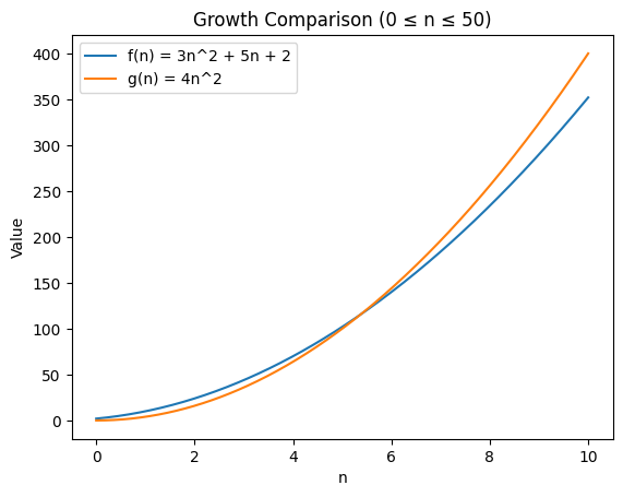
Therefore, there exist constants and such that

and hence .

Here is another way to show . Suppose

where is some constant, then .

Example.
Let and . Then

Therefore, .

Example.
Let and . Then

Using the fact that as , we get

Hence, .

If you wonder how we get as , recall from calculus that logarithmic functions grow more slowly than any positive power of . In particular, we can use L’Hospital’s rule:

Thus, grows strictly slower than , and hence as .

Definition.
We say if there exist constants and such that

Alternatively, this means .