The Role of Mathematical Models in Modern Cancer Therapy
By Shivali H. Patra and Wenhao Lu
Introduction
Cancer is not a single moment or a sudden mistake. It is a biological process that unfolds over time. Tumors grow over time, pressing into nearby tissue and drawing resources away from healthy cells, all while slipping past the immune system meant to stop them. As treatments are introduced, cancer does not simply disappear. Some cells survive and change, finding ways to resist what once worked against them. This is why cancer can return, even after aggressive therapy. Understanding cancer as an evolving process, rather than a single event, helps explain both the difficulty of treating it and the need for new approaches.
Traditionally, doctors have relied on imaging, biopsies, and population-level clinical trials to decide how and when to treat cancer. While these tools are essential, they often provide only snapshots of a much more complex and constantly changing system. This is where mathematics becomes more valuable. By combining biological knowledge with mathematical models, researchers can simulate how tumors are likely to grow, respond to therapy, and develop resistance, before those outcomes occur in a patient’s body.
The Math Behind It
The goal of mathematical oncology, which applies mathematics and computer modeling to study how tumors grow and respond to therapy, is not to replace biology or clinical judgment, but to strengthen them. When biological mechanisms are translated into equations, doctors gain a way to test treatment strategies safely, personalize care, and avoid unnecessary harm. In order to mathematically model tumors, they are treated as a dynamic system whose behavior can be described and predicted using equations. Researchers use mathematics rather than observation or trial-and-error in order to formalize how tumors are able to respond to drugs and evolve over time. This allows treatment strategies to be tested computationally and for people to make predictions that would be impractical or unethical to directly test on patients.
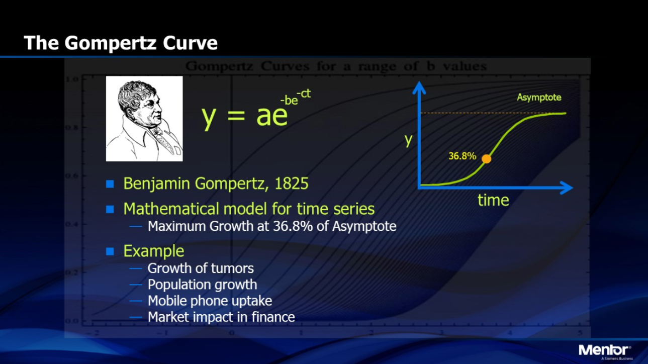
The foundation of math modeling for tumors and their growth is in differential equations, which describes how a quantity changes over time. In the context of tumor growth, a differential equation models how fast a tumor grows at any given time based on its current size. One example is the exponential growth model, which assumes the growth rate is directly proportional to the size of the tumor and thus predicts unlimited growth. However, simple exponential models fail because they ignore biological limits, so these more realistic models are used. Logistic growth equations capture the slowing of tumor growth as resources become scarce, while Gompertz models describe rapid early growth followed by saturation over time. These equations contain parameters such as growth rate and carrying capacity that are estimated from data and can forecast future tumor behavior with surprising accuracy.
Tumors’ drug resistance can be modeled using evolutionary and stochastic mathematics, where stochastic is the explicit inclusion of randomness into the model. Here, tumors are treated as competing populations of sensitive and resistant cells whose proportions can change under selective pressure from treatment. Stochastic models show that even very small resistant subpopulations can survive under different therapies and allow researchers to predict when and how resistance will emerge. Adaptive therapy naturally follows from this mathematical framework, in which models show that a controlled tumor population can suppress resistant cells by preserving competition. This is important because it enables mathematically optimized strategies that can prolong treatment effectiveness and ultimately improve patient outcomes.
Finally, mathematical models can become clinically useful when personalized. For example, patient-specific imaging and biopsy data are used to estimate the parameters in the math models through optimization and statistical inference. Optimization finds the parameter values that best fit the observed patient data, and statistical inference uses the data to quantify uncertainty and make conclusions about the model’s predictions. Once calibrated, these individualized models can predict tumor growth trajectories, responses to treatments, and timelines for resistance in a specific patient, ultimately transforming cancer treatment from a generalized protocol into a personalized system through mathematical modeling.
Biological Interpretation: What the Math Represents in Real Tumors
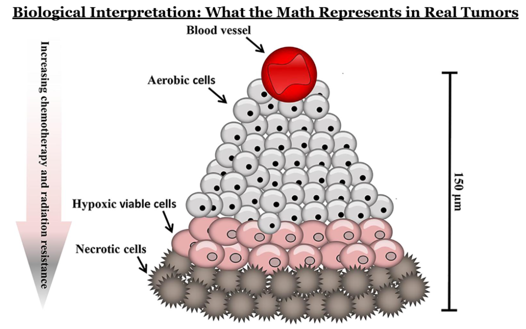
Behind every equation in tumor modeling is a biological process. Logistic and Gompertz growth curves reflect the fact that cancer cells depend on oxygen, nutrients, and physical space. As a tumor grows, its inner regions often become starved of oxygen, creating hypoxic cores that slow growth but also make cancer cells harder to kill. These biological constraints explain why tumors rarely grow indefinitely at the same rate.
Drug resistance emerges not because cancer cells “decide” to resist treatment, but because therapy creates an environment where only the most adaptable cells survive. Resistant cells may already exist in small numbers before treatment begins. When sensitive cells are killed, resistant ones are left behind to expand. Mathematical models capture this, which in turn helps researchers understand why aggressive treatment can sometimes accelerate resistance rather than prevent it.
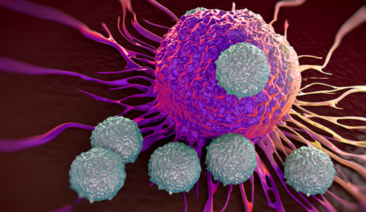
The immune system adds another layer of complexity. Tumors constantly interact with immune cells such as T cells. Sometimes these interactions activate the immune response, and other times they suppress it. Feedback loops involving cytokines can strengthen immune activity or cause it to collapse altogether. Mathematical models based on predator–prey biology help explain immune exhaustion and why immunotherapies such as checkpoint inhibitors work well for some patients but not for others. In these models, immune cells, such as T cells are treated as “predators” that attack cancer cells, while tumor cells act as the “prey.” Initially, immune cells may successfully suppress tumor growth, but prolonged exposure to cancer can overstimulate them, causing immune exhaustion, a state in which immune cells lose their ability to effectively kill cancer cells. These models help explain why immunotherapies are not universally effective: checkpoint inhibitors work by reactivating exhausted immune cells, but if immune suppression is too severe or if tumors evolve ways to avoid immune detection, the treatment may fail.
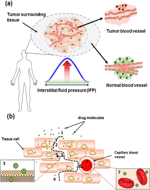
Spatial models add another important layer by accounting for the physical structure of tumors. Unlike simpler models that assume tumors are uniform, spatial models describe how cancer cells, blood vessels, oxygen, and drugs are unevenly distributed throughout a tumor. Because some regions have poor blood supply, drugs may not reach all areas equally, allowing cancer cells in protected regions to survive treatment. This uneven drug exposure helps explain why combination therapies that are using drugs to penetrate tumors in different ways or target different regions are often more effective than single-drug treatments.
The Impact in Clinical Terms
However, the true power of mathematical modeling lies in personalization. When a patient’s imaging data, biopsy results, and treatment responses are used to calibrate a model, predictions become patient-specific rather than theoretical. Doctors can estimate how fast a tumor is likely to grow, when resistance may appear, and how different treatment schedules might change the outcome.
Importantly, these models support adaptive therapy, an approach already being tested in clinical trials. Instead of trying to eliminate every cancer cell at once, adaptive therapy uses biologically informed dosing to keep resistant populations under control. This strategy is grounded in both evolutionary biology and mathematics, showing how interdisciplinary approaches can extend patient survival.
Conclusion
Cancer is biological, but it is also predictable in ways that biology alone cannot always reveal. Mathematical models turn complex cellular behaviors into tools that help doctors think ahead rather than react after the fact. By combining tumor biology, immunity, and patient-specific data, mathematics allows researchers to explore treatment strategies safely and efficiently.
As these models continue to improve, they offer a future where cancer treatment is not just reactive, but anticipatory and designed around how a tumor is likely to behave, not just how it looks today. In that sense, mathematics does not remove the human element from cancer care; it strengthens it by helping treatments become smarter, safer, and more personal.
References
Arredondo, J. A., & Rivera, A. (2025). Recent advances in ODEs modeling of tumor-immune responses: A focus on delay effects. Mathematical Biosciences and Engineering, 22(12), 3060–3087.
Benzekry, S., et al. (2014). Classical mathematical models for description and prediction of experimental tumor growth. PLoS Computational Biology, 10(8), e1003800. https://doi.org/10.1371/journal.pcbi.1003800
Kamran, M., et al. (2025). Mathematical modeling and analysis of tumor growth models integrating treatment therapy. Mathematical and Computational Applications, 30(6), Article 119. https://doi.org/10.3390/mca30060119
Vaghi, C., et al. (2020). Population modeling of tumor growth curves and the reduced Gompertz model. PLoS Computational Biology, 16(1), e1007178. https://doi.org/10.1371/journal.pcbi.1007178
Yin, A., et al. (2019). A review of mathematical models for tumor dynamics and treatment resistance evolution of solid tumors. Frontiers in Oncology, 9, Article 1371. https://pubmed.ncbi.nlm.nih.gov/31250989/