Consider a geometric Brownian motion driven by the Stochastic Differential Equation (SDE)
where is a canonical Brownian motion on a probability space . The process is often used as the most basic model of stock prices in real time. Here we will motivate the problem by considering as the population of an invasive species that has found its way into a new habitat where resources are plentiful. The lack of scarcity means that the population will not come close to the carrying capacity of its habitat on the time scale we are interested in, hence we can use Eqn. () to model its growth instead of a more complicated logistic type model.
The stochastic process is the strong solution to the SDE in Eqn. (). Since the deterministic growth rate of is , it is natural to consider the quantity . is the ratio between and the population that would result from a model of deterministic exponential growth. We may then ask, what is the probability that ever becomes twice, three times, or times as large as a its deterministically governed counterpart? In other words, we would like to characterise the function paying especial attention to the limit . We can obtain an easy bound on by noting that is a non-negative martingale with for all , hence Doob’s martingale inequality for reads
For this bound is trivial, but,as we will see, it is the best constant-in- bound for when . For the time being we will focus on the case .
If we define then is equivalently written as
Here let us state two very useful results without proof. The first gives us the density of the running maximum of Brownian motion. This is not so difficult to prove, and I hope to make a separate post about it very soon. The second is a simplified version of Girsanov’s theorem which will serve our current needs well enough.
To state the next result we introduce the notation for the quadratic variation of up to time , and we write for the covariation of andNotice that if we set , then
so that . We will now use these two results to calculate . First note that since a.s. for all , and hence, by the Radon-Nikodym theorem, exists and is given by Setting we have where in the last equality we have used the fact that is the joint density of and under (since is a BM under ).
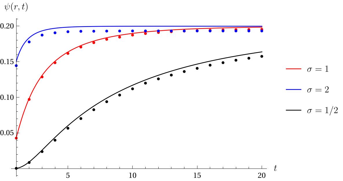
Below is a plot of the analytic solution from Eqn. () in the case with numerical results obtained by sampling the process at regular intervals. The numerics systematically underestimate the true probability because sampling the process underestimates the maximum . This raises another question: Does the discrete time process converge to ? In what sense? And how quickly? A topic for another day.
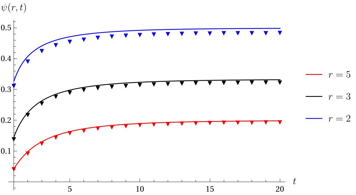
We can see that is, of course, non-decreasing: If at time , has had an excursion outside of then what happens later doesn’t matter. If it has not had such an excursion, then it may do in the future. The concavity of is intuitively explained when we remember that for long times, hence as . So if the event is observed then probably exceeded at some moderately small time. Indeed, it appears from the plots that as . To see that this holds for all write We have skipped a few steps in arriving at the last equality, but these steps just involve completeing the square inside the exponential which is standard. We will now cheat a little by using Mamthematica to evaluate this last integral, which gives where is the complementary error function Since , the limit falls out easily from Eqn. (). We will leave it to the reader to check that is an increasing function of . The monotonicity of and the limit together imply that the bound in Eqn. () is the best bound that is constant in .
We can also get a handle on the rate of convergence in Eqn. () by using the well-known Mill’s ratio inequalities, for all . Let and apply Mill’s inequalities to Eqn. () to find Since , Eqn. () implies that . So larger values of will result in faster convergence to the limit; see the figure below.