Demystifying the Black Box: Mastering Analog Signals with the Three Golden Rules of Op-Amps

Capturing clean, meaningful data from the physical world is notoriously difficult. Whether you are sampling a weak biological pulse, capturing acoustic vibrations from a microphone, or reading sub-millivolt variations from a bridge sensor, real-world signals are inherently fragile. They are plagued by environmental noise, vulnerable to loading effects, and often too faint for a microcontroller’s Analog-to-Digital Converter (ADC) to resolve.

To bridge this gap between the chaotic analog world and digital processors, engineers rely heavily on the operational amplifier, or op-amp.

An op-amp is a high-gain, direct-coupled voltage amplifier featuring two differential inputs (inverting and non-inverting) and a single-ended output. For many junior engineers and students, however, the op-amp behaves like an intimidating “black box” full of internal transistor topologies, parasitic behaviors, and dense textbook mathematical derivations.

Fortunately, you do not need to calculate individual transistor bias currents to design practical circuits. By treating the component as an “ideal” device governed by the Three Golden Rules, you can dramatically simplify circuit analysis and design highly predictable analog front-ends.

What is an Ideal Op-Amp?

Where represents the open-loop voltage gain, is the voltage at the non-inverting terminal, and is the voltage at the inverting terminal.

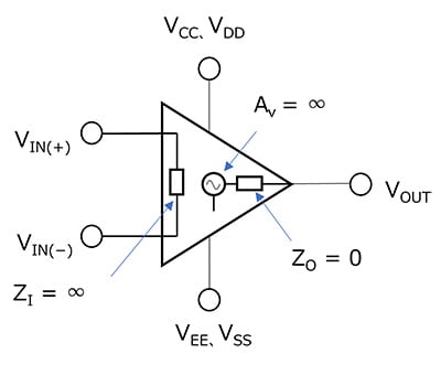
In an ideal operational amplifier, we assume three impossible, although highly practical conditions:

1. Infinite Open-Loop Gain (): The smallest differential input splits open to a massive output swing.

2. Infinite Input Impedance (): The input terminals draw absolutely zero current from the surrounding circuit.

3. Zero Output Impedance (): The output can source or sink unlimited current without its voltage dropping.

From these baseline assumptions emerge the operational strategies popularized by classical literature such as Horowitz and Hill’s The Art of Electronics. Let’s break down these foundational guidelines.

Rule 1: The Virtual Short Circuit Condition

When an op-amp is configured in a closed loop with negative feedback, the output adjusts to force the differential input voltage to zero. Choosing to use negative feedback leads to a simple identity: Why does this happen? Think of negative feedback as a self-correcting equilibrium loop. If increases slightly above , the huge open-loop gain causes to shoot upward. Because a fraction of this output is routed back to the inverting input (), climbs until it perfectly matches . Consequently, the two input terminals copy each other’s voltage, establishing a “virtual short.” They act as if they are shorted together for voltage, yet no physical current passes between them.

Rule 2: The Infinite Input Barrier

The input terminals draw absolutely zero current from the source.

Because the internal architecture of an ideal op-amp features an infinite input impedance, it acts as an absolute physical wall to electrons. This rule is vital for signal preservation. If an analog sensor has a high internal source resistance, drawing current from it will cause a severe voltage drop across its internal resistance (known as loading error). Because the op-amp draws zero current, it samples the raw, unadulterated voltage of the sensor without altering it.

Rule 3: Zero Output Impedance

The output terminal acts as a perfect voltage source, capable of delivering any current necessary to maintain its voltage.

Real-world filters and downstream digital stages require driving power. An ideal op-amp can drive heavy resistive or capacitive loads without its output voltage sagging. This decouples the input stage from the output stage, allowing engineers to cascade multiple circuit blocks cleanly as outlined in Texas Instruments’ Op Amps for Everyone handbook.

Practical Multiplier: Analyzing the Inverting Amplifier

Let’s use these golden rules to analyze one of the most widely used circuits in analog electronics: the Inverting Amplifier.

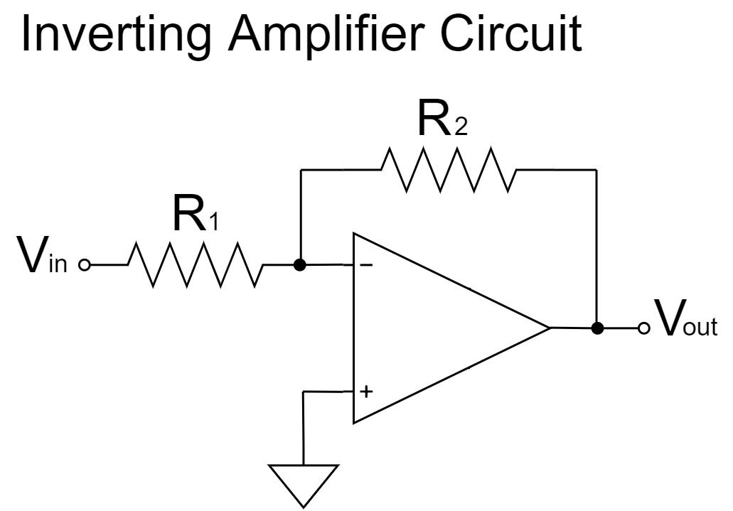
In this circuit, the input signal is applied through resistor to the inverting input (). A feedback resistor connects the output back to . The non-inverting input () is tied directly to the system ground.

We can derive the entire closed-loop voltage gain equation using only our golden rules and basic Kirchhoff’s Current Law (KCL):

1. Apply Rule 1 (Virtual Short): Since is grounded, the inverting node must also sit at ground potential. Therefore, . This node is commonly referred to as a virtual ground.

2. Apply Rule 2 (Infinite Input Impedance): No current enters the inverting terminal. Therefore, the current flowing through from the input signal () must pass entirely through the feedback resistor to reach the output (). This leaves us with the baseline equality .

To tie it all together, we write Ohm’s Law for both branches, equate the currents, and solve for the total circuit gain:

Equating equation and equation gives the final relationship:

By applying the golden rules, the massive, unpredictable open-loop gain () disappears entirely from the equation. The circuit’s overall gain becomes completely stable, relying strictly on the ratio of two physical resistors ().

The Real-World Hardware Perspective

While the ideal rules are indispensable for structural planning, physical silicon devices introduce limitations. Modern precision applications demand single-supply components capable of matching these ideal assumptions as closely as possible.

A prime industrial example is the Texas Instruments TLV2782, a dual-channel, operational amplifier optimized for battery-powered, high-fidelity signal acquisition.

Analyzing its architecture reveals how close modern manufacturing comes to the ideal constraints, alongside the operational parameters you must accommodate:

• Rail-to-Rail Input and Output (RRIO): Unlike older legacy chips (such as the LM741) which clip signals if they get within a few volts of the power supply rails, the TLV2782 features rail-to-rail capabilities. This enables maximum dynamic voltage range on low-voltage (1.8 to 3.6) microcontroller supplies, keeping the virtual short condition valid across almost the entire supply spectrum.

• The High-Impedance Reality: The TLV2782 utilizes CMOS input transistors. As explored in comprehensive circuit primers like Sergio Franco’s Design with Operational Amplifiers and Analog Integrated Circuits, this yields an exceptionally high input resistance, restricting the input bias current to a minuscule pico-ampere () scale. For lower frequency instrumentation, it effectively acts as a perfect infinite barrier.

• Bandwidth and Gain Limitations: In the physical world, gain drops off as signal frequency increases. The TLV2782 features a Gain-Bandwidth Product (GBW) of 8. If you design a high-gain stage, you must monitor your signal frequencies to ensure the open-loop gain remains high enough to sustain the virtual short assumption.

Conclusion: Turning the Unknown into a Predictable Tool

The operational amplifier does not need to remain a mysterious black box. By anchoring your designs around the Three Golden Rules (virtual short circuits under negative feedback, zero input current draw, and robust output driving capability), you can comfortably analyze, simulate, and wire complex analog systems.

Once you understand how these rules mandate component behavior, you can leverage precision hardware to filter out real-world noise, buffer sensitive transducer signals, and construct robust, predictable circuits ready for downstream digitization.

References

Allelco. (2023, July 24). TL082 dual JFET op-amp pinout, equivalents, and applications. Allelco Electronics Blog. https://www.allelcoelec.com/blog/TL082-Dual-JFET-Op-Amp-Pinout,Equivalents,and-Applications.html
Franco, S. (2015). Design with operational amplifiers and analog integrated circuits (4th ed.). McGraw-Hill Education. https://www.mheducation.com
Horowitz, P., & Hill, W. (2015). The art of electronics (3rd ed.). Cambridge University Press. https://www.cambridge.org/academic/subjects/engineering/circuits-and-systems/art-electronics-3rd-edition
Mancini, R. (Ed.). (2002). Op amps for everyone (Technical Report SLOD006B). Texas Instruments. https://www.ti.com/lit/an/slod006b/slod006b.pdf
Spiceman. (2022, November 8). Inverting amplifier circuit with LTspice simulation examples. Spiceman Analog Circuit Academy. https://spiceman.net/inverting-amplifier-circuit/
Texas Instruments. (2005, January 14). Family of 1.8 V hi-speed rail-to-rail I/O operational amplifiers with shutdown (Rev. E) [Datasheet]. https://www.ti.com/lit/ds/symlink/tlv2782.pdf?ts=1781509289993
Toshiba Electronic Devices & Storage Corporation. (2024). What is the ideal op-amp?. Linear Op-Amp Knowledge Base Frequently Asked Questions. https://toshiba.semicon-storage.com/us/semiconductor/knowledge/faq/linear_opamp/what-is-the-ideal-op-amp.html