Special thanks to my friend Ming from Gauntlet for his helpful reviews and points that I have incorporated here.
Why This and Why Now?
A long time ago, I used to be knee deep in risk management in DeFi. I am now trying to become more of an Adversarial Market Design and Consensus guy but I always wanted to write about the purely technical bits of DeFi risk management once. Here’s a small exercise in doing so. I am keeping this mostly as an engineering post that is implementable than a math post although you’ll have to deal with some math in the beginning.
The Set Up
Assume that there is some token . follows an unknown stochastic process (), with (). has an economic system that is one of the factors informing its price along with some erratic bounded rationality behaviour and arbitrage trades that determine its price movement (the space of factors is infinite so we will not care about too much rigour here).
Let the price points be assumed to be random samples dependent on time that will be its price trajectory.
At each time , the token price has a marginal distribution , but the object of interest is the full path distribution over trajectories: A Monte Carlo simulation samples possible price trajectories from this path distribution:
How do we do it?
Mathematically? Go crazy. There’s all sorts of models from stochastics that are usable however this blog post is about practical implementations with an emphasis on computational hardness. Different people may think differently about this.
Way I see it, there’s at least two approaches you can start up right now: Optimization and Statistical Inference (The two approaches are not mutually exclusive). Intuitively, optimization is more about going towards to parameter of least loss by trying different approaches and statistics is more about taking samples of data to derive the model that may fit best. In my experience optimization approaches are usually computationally expensive yet more accurate and statistical approaches are usually less accurate but quicker.
A practical Monte Carlo system usually has two layers
The first layer is statistical calibration. We observe historical price data, returns, volatility, liquidity, oracle behavior, protocol revenue, TVL, liquidations, and other relevant variables. Then we choose a stochastic (or linear??) model whose parameters can be estimated from this data.
The second layer is optimization or control. Once we can generate simulated price paths, we can ask what action performs best across those paths.
Let’s do it!
Suppose a vault manager is deciding how much capital to allocate to token . The goal is not to predict the exact future price but rather to estimate a distribution of possible future paths and allocate capital accordingly.
Start with the log returns (since log returns are usually approximated to be normally distributed - huge huge huge discourse here):
Assume returns are partly explained by observable state variables:
If the residuals are approximately well behaved, the production system can start with a simple linear model:
The model is not assumed to be true forever. It is just the cheapest useful approximation. Candidate models can be compared using AIC and BIC:
where is the number of parameters, is the sample size, and is the maximized likelihood. Lower means a better tradeoff between fit and complexity.
Ming’s point: Practically Correlograms are a particularly useful method to visually check for optimal candidate as well.
Once the model is selected, simulate forward. For each Monte Carlo path ,
where
Run this 1000 times to produce 1000 possible future price paths:
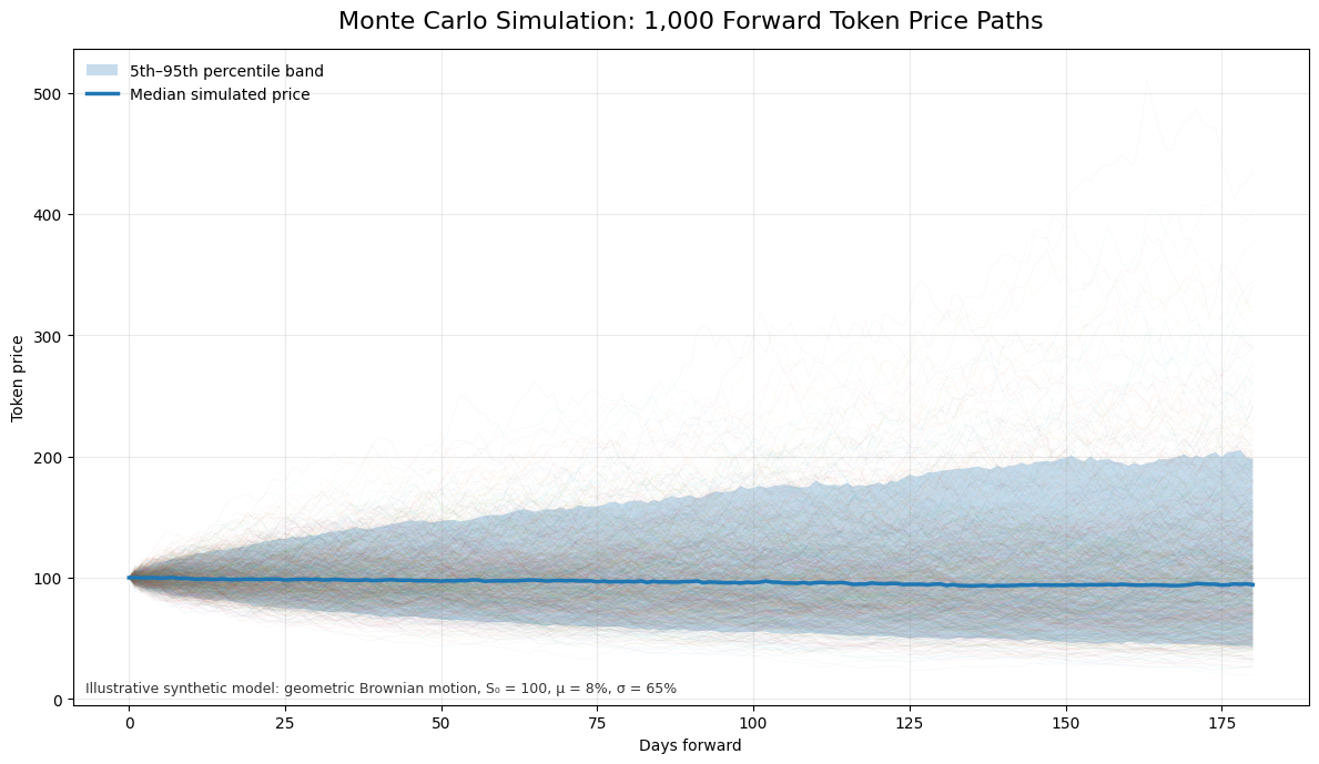
The vault manager then looks at a simple allocation rule: if the bottom 5% loss is too large, reduce allocation. If there are more paths towards profit then loss, increase allocation to howsoever the profit is increasing to. The allocation is updated every training epoch which is hourly, daily, or weekly depending on latency needs and data quality.
The Kelly Criterion would be a good measure too but managers should probably move towards the bayesian side more here since the priors keep changing in these environments.
Now the Meat
Okay, I get it, I only use math all the time and it isnt useful. I’ll have to talk about how to do it too.
Let us assume that there exists a block indexed price data service where the service exposes an HTTP GET endpoint returning the token price at that block that will give us a JSON response which may include (but not limited to) the following:
{
    "token_hash" : "0xabcd...",
    "block_number" : XXXXXXXX,
    "token_price" : P,
    "timestamp" : "YYYY-MM-DDTHH:MM:SSZ"
}
Of course a ranged GET query will give us the token price over a period of blocks which will form the dataset over the range of time that we have been looking for.
Cleaned dataset will look like a hashmap (with indexing in case time series models) or an array like
[P_1,P_2,....,P_t]Now the prices will be differenced (to get returns) and logarithmically scaled and we use the returns data instead because raw token prices are often nonstationary, while log returns are usually a better input for short-horizon statistical modeling and Monte Carlo simulation. Therefore our final data:
[r_2,r_3,....,r_t]where log returns
Now that the data has been dealt with, we run it into our linear model with AIC and BIC optimized parameters.
For the statistical model, suppose we fit a family of linear autoregressive models:
Each lag order gives a different candidate model. We estimate the parameters first, then compare the fitted models using AIC or BIC.
Pseudocode for the Curious
This is pseudocode for the model fitting which is heavily expensive as the lags are varied
Input:
    candidate_lags = {1, 2, 5, 10, 20}


For each lag order p:

    Build regression dataset:
        r_t = β_0 + β_1 r_{t-1} + ... + β_p r_{t-p} + ε_t

    Estimate β using OLS or maximum likelihood.

    Compute residuals.

    Compute log-likelihood.

    Compute AIC and BIC.

Select the model with the lowest AIC or BIC.

Use the selected model and residual distribution as inputs to Monte Carlo simulation.
To write out the code for the model inference is a seperate post altogether including all the implementations and improvements. Similarly for Monte carlo simulation
Input:
    selected_model
    recent_returns = [r_{T-p+1}, ..., r_T]
    latest_log_price = x_T
    num_paths = M
    horizon = H


For each Monte Carlo path i = 1 to M:

    Set current_log_price = x_T.

    Set return_history = recent_returns.

    For each future step h = 1 to H:

        Predict next return:
            r_hat = β_0 + β_1 r_t + ... + β_p r_{t-p+1}

        Sample random shock:
            ε_h ~ selected_residual_distribution

        Simulate next return:
            r_sim = r_hat + ε_h

        Update log-price:
            x_next = current_log_price + r_sim

        Store x_next.

        Update return_history with r_sim.

        Set current_log_price = x_next.


Convert simulated log-prices back to prices:
    P_sim = exp(x_sim)
Computationally, the expensive part is : simulating paths over future steps, although this is highly parallelizable because each path is independent. A great resource to read for this is here.
The final output is a distribution of possible future prices, from which we extract risk metrics such as downside quantiles, probability of loss, VaR, and expected shortfall.
Complexity, Scaling, and Latency for the Curious
Let:
= number of price observations
= number of candidate models
= maximum lag order
Data Cleaning is linear and scales linearly with the data queried:
Constructing log-prices and log-returns costs:
Fitting one linear model costs approximately:
as per sources on the internet about how Python libraries do it. Still pretty high ngl.
Fitting candidate models costs:
Once the best model is chosen, Monte Carlo simulation adds another cost. Each simulated path has future steps, and each step evaluates a -lag model, so the simulation cost is
If is small and fixed, this is usually written as
Therefore the full cost is approximately
The memory cost is for the price and return arrays. If the full regression matrix is stored, memory becomes . If all Monte Carlo paths are stored, simulation memory is but as we are smart people we only store final outputs and this can be reduced to or less.
This scales well because the expensive jobs are independent. Different tokens, windows, lag orders, and Monte Carlo paths can run in parallel (Monte Carlo Simulations are called “Embarrassingly Parrallel” haha).
Ming’s point: block level data can be too noisy. Indeed I agree with it. When you query a block level price data service, it will usually be the case that the prices of tokens are usually extremely similar in consecutive blocks which do not provide any additional information on price behaviour. A good solution that he proposed and I agree with is resampling across a large set of data to get decrease granularity (but increase information) and use that instead. You won’t have as much data but you will have more information plus more computational strength. Of course resampling adds a mild time complexity too which increases the calibration time however improves accuracy across long time horizon
In practical terms, this is very manageable on a personal scale especially using multithreading techniques. On a standard 8-core machine with 16–32GB RAM, a run with observations, candidate models, , Monte Carlo paths, and steps should usually finish in seconds once the data has been queried.
At larger scale, say many tokens, rolling windows, and paths, the job should move to cloud workers. The good news is that both calibration and simulation split cleanly across tokens, models, windows, and paths, so a small cloud cluster can turn a job that takes minutes into at most one minute batch job. The final output is a distribution of future prices and risk metrics such as worst quantiles, VaR, expected shortfall, and probability of loss.
Always Remember
The main production rule:
Full Statistical Inference should be a scheduled batch job. The live vault system should only load the latest calibrated model, update the current price state, run the forward simulation, and return the risk estimate. If you ask me for tech stack, Julia is well suited for calibration and simulation because it is strong in numerical computing and parallel Monte Carlo. Go or Rust is better for the production API, orchestration, and low latency service layer and I’d add some third party cloud infra like AWS for computational overhead along with a Grafana monitoring system to check for crashes.
I’ll go deeper into the tech stack if people like it!! Thanks for reading.
I have been Abhimanyu Nag