Linear Regression From Scratch: Mastering the Fundamentals 🚀
Linear Regression is often the first algorithm encountered by
aspiring data scientists. It’s simple, interpretable and forms the basis
for more complex models. It can be easily implemented using the
scikit-learn library, but to truly understand the
mathematical foundation behind the model, we will implement it from
scratch. In this post, we will:
understand the intuition behind the linear regression
derive the gradient descent update rules
implement the model in Python from the ground up
visualize the model’s loss
compare our custom model’s performance to the scikit-learn model
What is Linear Regression
At its core, linear regression models the relationship between one or more independent variables () and a dependent variable () by fitting a straight line. This model is given by the mathematical equation where:
is the predicted value of the dependent variable
and are the parameters of the model, weight (or slope) and bias (or intercept) respectively
Our goal is to minimize the error between the predicted values and the true values .
Cost Function: Mean Squared Error (MSE)
The quality of the model’s predictions is measured using the Mean Squared Error function defined as: Where:
is the number of training examples
is the predicted value of the training example
is the true value of the training example
Optimization: Gradient Descent Update Rules
To minimize the cost function, we use gradient descent, an algorithm that iteratively updates the parameters and in the direction that reduces the loss. The update rules are
Where:
is the learning rate which controls the step size of each update
Gradients are calculated as:
Implementation in Python
Step 1: Importing libraries
    import numpy as np
    from sklearn.preprocessing import StandardScaler
    import matplotlib.pyplot as plt
    import seaborn as sns
    from sklearn.model_selection import train_test_split
Step 2: Define the linear regression class
    class LinearRegressionScratch:

    def __init__(self, learning_rate=0.01, n_iterations=10000):
        self.learning_rate = learning_rate
        self.n_iterations = n_iterations

    def fit(self, X, y):
        self.n, self.m = X.shape # self.m is the number of features, self.n is the number of samples
        self.w = np.zeros(self.m)
        self.b = 0
        self.X = X
        self.y = y
        self.losses = []

        for i in range(self.n_iterations):
            self.update_params()
            self.update_params()
            loss = self.compute_loss()
            self.losses.append(loss)  # Record the loss

        return self

    def update_params(self):
        y_pred = self.predict(self.X)

        # compute gradients
        dw = (1/self.n) * np.dot(self.X.T, (y_pred - self.y))
        db = (1/self.n) * np.sum(y_pred - self.y)

        # update parameters
        self.w -= self.learning_rate * dw
        self.b -= self.learning_rate * db

        return self, dw, db

    def compute_loss(self):
        y_pred = self.predict(self.X)
        loss = (1/(self.n)) * np.sum((y_pred - self.y) ** 2)
        return loss

    def predict(self, X):
        return np.dot(X, self.w) + self.b
Step 3: Train and Evaluate the model
To ensure faster convergence and stable optimization, the input features
were standardized using Scikit-learn’s StandardScaler.
📊 Data: Auto MPG Dataset
🎯 Goal: Predict a car’s fuel efficiency (mpg) using engine and car specs.
🔗 Source: Available in seaborn or directly via UCI ML repo.
    data = sns.load_dataset("mpg").dropna()

    # we use one feature and one target variable
    df = data[["horsepower", "mpg"]]
    # define X and y
    X = df[["horsepower"]].values.reshape(-1, 1) # It reshapes a 1D array into a 2D column vector
    y = df["mpg"]

    # split the data into training and testing sets
    X_train, X_test, y_train, y_test = train_test_split(X, y, test_size=0.2, random_state=42)

    # standardize the data
    scaler = StandardScaler()
    X_train = scaler.fit_transform(X_train)
    X_test = scaler.transform(X_test)

    n = X_train.shape[0]
    m = X_train.shape[1]

    # create an instance of the VickLinearRegression class
model = LinearRegressionScratch(learning_rate=0.01, n_iterations=1000)

    # fit the model to the training data
    model.fit(X_train, y_train)

    # make predictions on the test data
    y_pred = model.predict(X_test)
Visualizing the fitted line and the loss curve
    # Visualize the fitted line on the training and test sets
    fig, ax = plt.subplots(1, 2, figsize=(14, 7))
    ax.flatten()
    ax[0].scatter(X_train, y_train, color = 'blue')
    ax[0].plot(X_train, model.predict(X_train), color = 'orange')
    ax[0].set_title('Training set: horsepower vs mpg')
    ax[0].set_xlabel('Horsepower')
    ax[0].set_ylabel('MPG')

    ax[1].scatter(X_test, y_test, color = 'blue')
    ax[1].plot(X_test, y_pred, color = 'orange')
    ax[1].set_title('Test set: horsepower vs mpg')

    ax[1].set_xlabel('Horsepower')
    ax[1].set_ylabel('MPG')

    plt.show()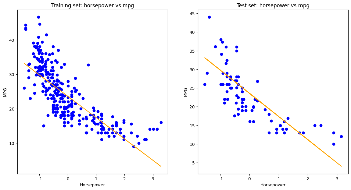
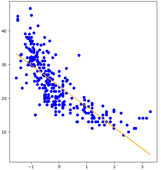
The fitted regression line closely aligns with the training and test data, capturing the negative correlation between horsepower and MPG. The consistency across both sets suggests the model generalizes well without overfitting.
    plt.figure(figsize=(8,5))
    plt.plot(range(model.n_iterations), model.losses, color='blue')
    plt.title("Loss Curve (Training Error vs Iterations)")
    plt.xlabel("Iterations")
    plt.ylabel("Loss (Cost Function J)")
    plt.grid(True)
    plt.show()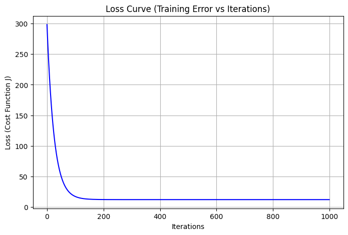
The loss curve shows a steep initial decline followed by a smooth plateau, indicating rapid learning and stable convergence. The absence of oscillations confirms that the gradient descent updates were well-behaved throughout training.
Comparison with the Sklearn benchmark
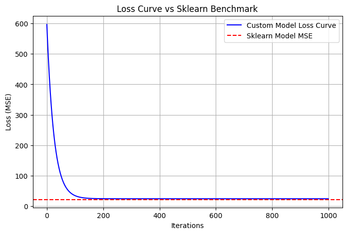
The custom model’s loss rapidly decreases and converges closely to the benchmark MSE from Scikit-learn, shown as a horizontal red dashed line. This alignment demonstrates that our from-scratch implementation achieves performance comparable to a well-established library.
What You’ve Learned
How linear regression model works
How to calculate gradients and implement gradient descent
How to code a working linear regression from scratch
How to visualize the results and loss convergence
Github Repository