Edit: new version
Here is a humble (and shy) attack on lwe with a binary secret and a gaussian error. It is inspired by the BKW attack, but it needs much less samples. Instead of selecting very rare vectors in a huge collections of vectors we manage to get the most information possible from each vector.
We present two codes, we will start with a simple attack on few bits and then we discuss an improvement to the first code.
To run the first program:
Install rust
in the Cargo.toml file, add
[dependencies]
rand = "0.9.0"
rand_distr = "0.5.1"
rayon = "1.10.0"
cargo run –release
The instructions for the second program are described later
Let’s start with the basic idea.
Basic principle
LWE
LWE is a a mathematical problem I will not detail too much here, you just need to know that it is at the core of several post quantum crypto system recently proposed for the reason that, at the time of writing those lines, there are no known quantum algorithm that could break them.
To sum it up (way too) quickly the LWE problem is a set of linear equations of size where all coefficients are being sampled uniformly, ( in theory, the problem is not defined over a ring, but in real life, it is). The collection of coefficients can be seen as a vector of . The secret is also a vector of , thus each linear equation can be seen as a scalar product between two vector of having their result in . will be called the secret key, because it usually constitutes the core of the private key for all crypto system relying on LWE.
Solving that system is easy, but the LWE problem modifies it slightly such that it becomes almost impossible to find the solution, unless becomes very large. Adding a small random error to each , leads to one of the toughest cryptographic problem to solve.
Problems in cryptography are often not very complicated, but they are hard. It is easy to find a way to solve LWE, yet it is very expensive in terms of computation to do so.
In an lwe sample, or its ring version, the last term is calculated as follow:
Usually follows a (discrete) gaussian distribution, but it is not mandatory. In cryptographic systems relying on LWE, the key is often taken in and not in . The attack presented heavily relies on that asumption.
BKW
The BKW attack on LWE relies on finding several vectors of LWE where the are all zero but one, and then average them. For example, if we wanted to find the first component, we would need to find vectors:
then sum those last components and divide the sum by in order to average them.
Those samples are very unlikely, the probability of picking up one is and the attack requires the average over the error to not wrap around the modulus, so needs to be small. The process has to be repeated for each component and thus the attack is very slow despite having a very fast treatment once the samples are obtained.
Alternatively finding samples with the same first non zero terms and averaging the different should lead to a value close to . (As long as is far enough from the representative bounds). To solve a system, We’re looking for different linearly independent vectors, and for each of these vectors, we need to find occurrences of that exact same vector. Finding several collisions among samples is less unlikely because of the "birthday effect", but we need to find n independent ones. Our method allows for finding "approximate" collisions, i.e. samples whose components are close to each others without being exactly the same. I suppose it might also be doable with the original BKW attack. One should consider the number of different values to be instead of , where is a spread around each component. When a collision is detected in our method, it is used to create a linear combination. It is insensitive to the representatives, and additions can provide new valid samples as well as subtraction, multiplying the number of collisions by 4 in a given set. One key difference between our method and the riginal BKW attack is that because all approximate collisions give rise to a new sample with small values, new collisions between aproximate collisions are increasingly more likely.
In the BKW attack, notable improvements can be obtained through linear combinations, yet the attack is still fairly slow and require a huge amount of samples.
Our proposition
We suggest several improvements over that method that allow to drastically reduce the number of initial samples and create a much faster attack overall. The attack relies on the asumption that the secret is distributed in and not in . The improvements are namely
Avoiding the modulus wrapping of the error problem.
Considering the scalar product as an error.
Using the Hamming weight.
Using the circular mean.
Step by step reducing the scalar product error through linear combinations.
Avoiding the modulus wrapping of the error problem
Avoiding the problem of the sum of the errors wrapping around the modulus is actually the easiest part. We just need to sum it in instead of . In practice we average over bits integers while is a bits integer.
Considering the scalar product as an error
Now that the wrapping of the sum of the error is no longer a problem, we can consider bigger errors. The error itself just needs to not wrap around the modulus. Thus we can consider the rest of the scalar product as an error.
where
As long as does not wrap around the modulus, and we select only such that is positive
If is negative, we can take instead, and add it to the calculation of the mean.
This is the principle behind the data treatment applied to selected samples:
You could wonder why it should work differently for different bits, since it seems we always add the same term. In reality we create a different mean for each because adding or is conditionned by the sign of
We create samples following an LWE (like) distribution, each of which is of size , the first terms are the s and the last term is .
We can have a great certitude that the scalar product lies in by selecting samples where the values of each is so small that it becomes very likely for the sum of the to land in .
For example, a radical solution to achieve such a feat is to set a limit on each such that the . Then the limit has the value:
Such a drastic constraint leads to very few samples being accepted, the probability of finding a random sample verifying this is
which is worse than exponential. If , it’s worse than . Happily, in most cases . Yet it is worse than which would be a brute force attack on the key.
We can already increase the number of acceptable samples by observing that on average, only half of the will participate to the scalar product. We increase the number of accepted samples by taking the hamming weight instead of . The hamming weight is the number of non zero bits of , thus . We usually have . Any large deviation of from can be used by the attack to recover the secret key more easily so we consider the hamming weight to be approximately .
the probability of finding a sample becomes
But because we do not know which is non zero, we just increase the detection threshold accordingly.
There are now
more samples now than in the case where all were considered. So we define a new limit
which is still terrible but much higher and gives a good estimate of the threshold we should use.
For and the limit for each individual becomes
Two key advantages appear here over the classical BKW attack.
The probability of finding a correct sample is much bigger than in the BKW attack
Each good sample can be used for any component
In addition, if we set a strict limit for each we miss all the sample which "almost made it". Some samples have coefficients all below the limit except for few of them, and those coefficient could very well count for nothing because could be equal to 0. Those samples can certainly be of statistical usefulness for computing an average.
The constraint we use instead is that the sum of the must be below a given threshold instead of constraining each component. Given that the negative terms often balance the positive terms and vice versa, having a sample that should be accepted is much more likely than with the previous constraint.
Calculating for we find a threshold :
The calculation of the mean over samples veryfying the constraint should then return
instead of as mentionned earlier
Distribution
Ideally, we might be able to increase further more the limit by studying more in detail the distribution of instead of . As previously stated the positive terms often balance the negative terms. grows like with a standard deviation growing proportionnal to while should grow like its standard deviation if its mean was to be . In our code that last constraint is not exactly verified because the mean is .
The distribution followed by a random variable where all are iid random variables following a uniform distribution over I uses the polynomial coefficients.
If where all the follows a uniform distribution , then the probability
where
is a polynomial coefficient, i.e. coefficient in front of when in the expansion of
Polynomial cofficients can be expressed as the sum of multinomial coefficients or by recurrence using the binomial coefficients.
(CAMILA C. S. CAIADO)
For the interval instead of we can shift all values and define a new variable , then
Because the polynomial coefficients are hard to compute, and because of the central limit theorem, when is big enough, we can fairly approximate those coefficients by a gaussian distribution of expected value ,
So what is the approximate probability that a random sample lies in the interval?
For this is . Approximately one third of all samples lie in . The problem is that our criterion on the sum of the can not pick up all samples landing in that interval.
On average , a reasonable heuristic is thus to have:
For this gives
But we already said on average, only half of the would be used so:
and
For , this gives an threshold actually lower than by using , .
In practice though, we recover lot of signal by setting a threshold around .
Back to our first idea to find the probability, we define new random variables for the following a uniform distribution . Then, if , then the probability to find a valid sample among random samples is
With and
For and , this gives a proability
Over 2000000 samples, we should recover approximately 22000. This is absolutely not the number of valid samples that we find, so there might be a huge mistake somewhere.
Hamming weight
We can further increase the number of samples by using some partial information about the key, namely the hamming weight of the key. The two techniques described here can be used for the other techniques described later.
If we know the hamming weight of the key, we can recover many more samples. In a real life situation, we might not know , but there are so few possibilities that if the attack is efficient, we might be able to simulate all the possible hamming weights brute forcing them, either on a single machine or on multiple machines. For a key of size , there are only different possibilities for the hamming weight, and the key not only is unlikely but is also not acceptable. The very same is true for . In that case, any sample would be valid if we would remove from , furthermore obviously, the keys with small or big hamming weights are easy to brute force.
Not small "small samples"
We previously explained that we were searching for samples where . Consider a sample where all values are "bigger" than but there exist a value such that
then knowing the hamming weight, we can transform the sample according to
and get a new valid sample verifying the constraint.
This is because
How many more samples can it represent? If we take a similar constraint than the one stated initially on each component of a vector, we need all values to verify .
Calling the smallest value of all the and the biggest value, if such exist then there is certainly one between and . Thus we require that . That condition can therefore be valid for any difference between any two components of the vector. Specifically we can apply that constraint to consecutive components.
We can thus require that
Since there are components instead of and the limit is twice as big as it was previously, the number of samples verifying that constraint is
bigger than with the previous calculation, which means we are more likely to find a sample knowing the hamming weight than when we do not know it. It seems that knowing the hamming weight provides more information than just reducing the key size by a single bit because the limit is twice bigger.
We take that factor for the probability of finding a valid sample
put some data here
There seems to be some sort of non sense here because it basically states that for all samples can become valid. Yet, it’s easy to verify that it is actually the case, which does not prove the model is valid per se.
Big hamming weight = small hamming weight
To recover a signal the algorithm piles up many , it takes advantage of the fact that . If instead, the algorithm works just the same, the values will average to where and where .
On the other side, it’s pretty obvious that it is easier to find a key with a small hamming weight than a key with a big hamming weight with the technique described. With a smaller hamming weight, is less likely to wrap around the modulus, thus the algorithm can accept samples with bigger components, hence more samples.
There is a way to handle big hamming weights just as small hamming weights. Let be a secret key of hamming weight . Then we can define
has a hamming weight , with components
Let
be a sample under the secret key then it’s easy to show that
A big hamming weight can thus be treated as a small hamming weight creating large negative values were the
circular mean
We already stated that if an LWE sample can be written:
then if is a constant,
is also an LWE sample.
For some constant and some representatives of the we can lower the disance . It’s then possible that a sample which previously did not verify the criterion
verifies
after finding the correct and the correct representative of the
Thus, knowing the hamming weight allows to transform the sample.After finding "the best" and "the best" representatives, applying the transformation to all samples change their distribution.
Let’s illustrate the idea by a small example with an error of . We choose the modulus to be with representatives initially in , , the secret key
if
the calculation of is detail is given by:
then the "mean" of all the is the sample is not "centered" around the mean. In addition, the distance to 0 is , the distance to its mean is .
Now if we are in a situation where we know the hamming weight of the secret key , then we can search for a smaller distance to the mean because we can transform .
To do so, we search for other representatives, compute the mean in that representative system and see if the distance to the mean is smaller than the distance we started with, here 24.
With respective means in of , , , , and distances to the mean of
The smallest distance to the mean is obtained by the third choice of representative whose mean is . So let’s ignore the fact that the mean is not an integer, and let’s take 8 as a mean. We now remove from all the of
Its distance to 0 is .
And to get a legitimate LWE sample, we also have to remove from .
The new sample is thus
We computed a sort of circular mean on the ring, and we centered the sample around that mean. The transformation on is performed such that the sample is still a valid LWE sample and we modified using the hamming weight. One important point to note is that sutracting the mean from all components expressed in other representative system move all the into the interval .
Here is an illustration of the procedure applied on the first components of the vector, keeping the treatment of for later.
:
:
:
After subtracting 8 to all the
:
Let’s try to evaluate how the distribution is transformed by the procedure described called roll_subarray in the code. We start with a vector where all are distributed uniformly over , the sample is the "best sample" by default, then the program
computes the mean in ,
computes the distance to the mean .
if the new distance is smaller than the best distance, the sample becomes the best sample.
looks to the "smallest" value and add to it.
repeat times
keeps the best sample and subtract the best mean to all . All values should belong to
On the ring, is either closer to the value just above or closer to the value just under, with a 50/50 probability. If is closer to than to then adding to decreases the spread between the maximal value and the minimal value. It might not diminish the distance to the mean, but in general, we expect that adding to the minimal value decreases the distance to the mean approximately half the time.
We model the situation by a probability to diminish or increase the distance to the mean at eahc step of the circular mean algorithm. The standard deviation of the number of times the distance can diminish is thus
The distance between two values is on average . A value is expected to be either closer to the above or the below with a chance of . We can expect to be uniformly distributed on an interval of span , so we can expect that if the distance diminishes at one step, it diminishes on average by a distance of .
Finally averaging on averages, after the complete procedure, we can expect to have a diminution of
For , this evaluates to
This is a very rough estimate because I do not have the exact distribution now. The procedure evaluates the total distance so we can also expect a similar influence on all the other values.
A better model but still unperfect, might be describing the situation by a random walk on a square grid of size where , where each node is a state that can be reached by a walker starting on one corner. At each step either increases or decreases. The walker is able to only go down right (for a lower value of the sum) or up right (for a greater value of the sum). The sum decreases or increases by a fixed amount at each step, and must return to its original value.
But that’s still not a perfect model, because it uses a fixed average distance of improvement. In the real world, the very last step of the roll_sub_array function can provide the smaller distance to the mean.
Hereafter are the distributions of the before and after the circular mean centering:
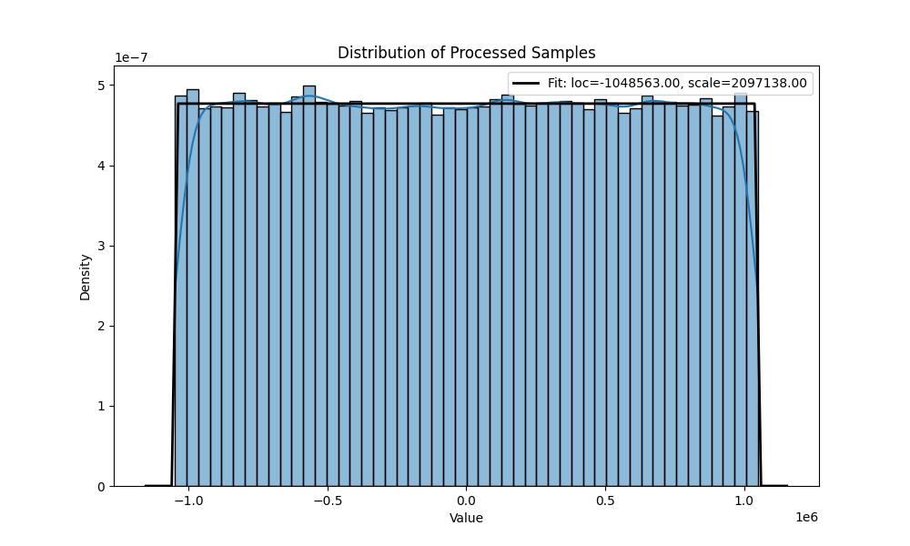
uniform distribution for and 10 000 samples.
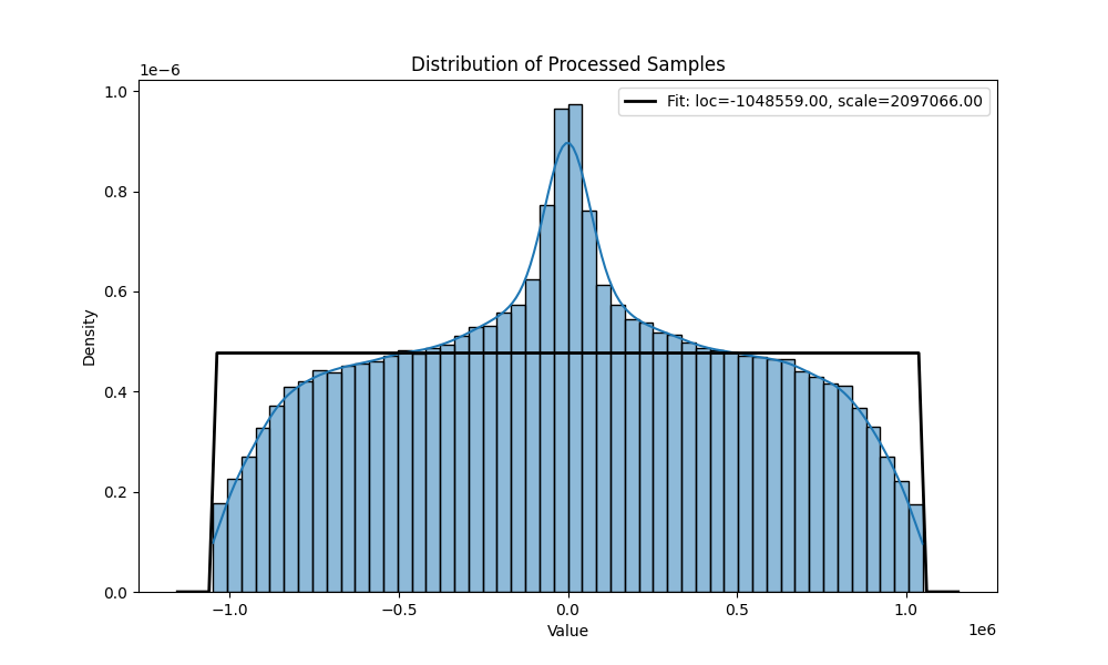
distribution after the transformation for and 10 000 samples.
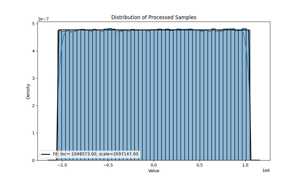
uniform distribution for and 10 000 samples.
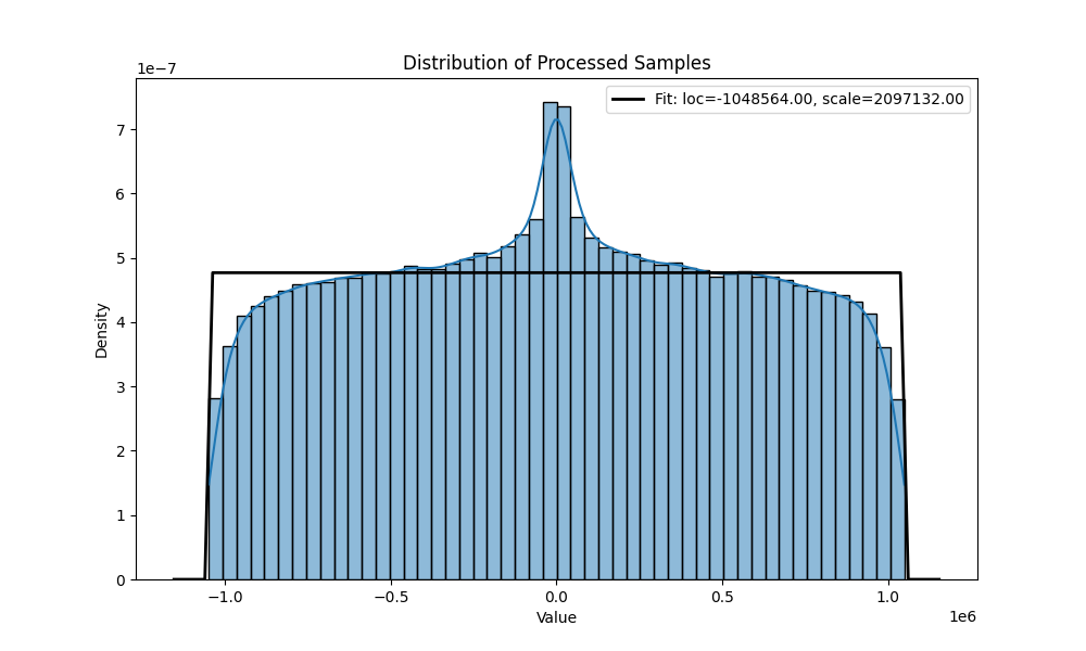
distribution after the transformation for and 10 000 samples.
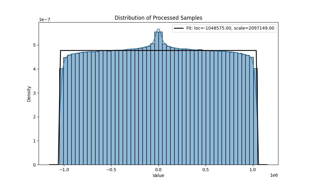
distribution after the transformation for and 10 000 samples.
Hereafter the evolution of the distance and the evolution of the minimal distance during the algorithm searching for the circular mean.
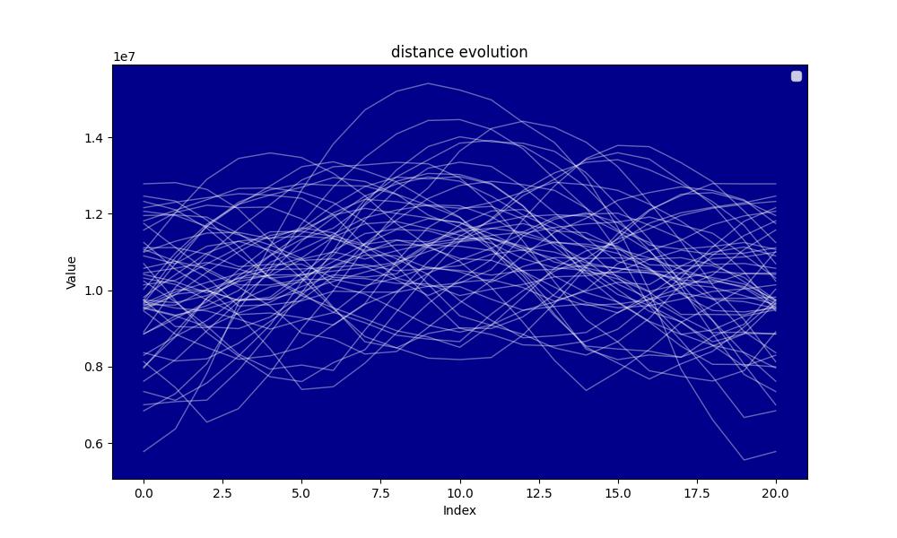
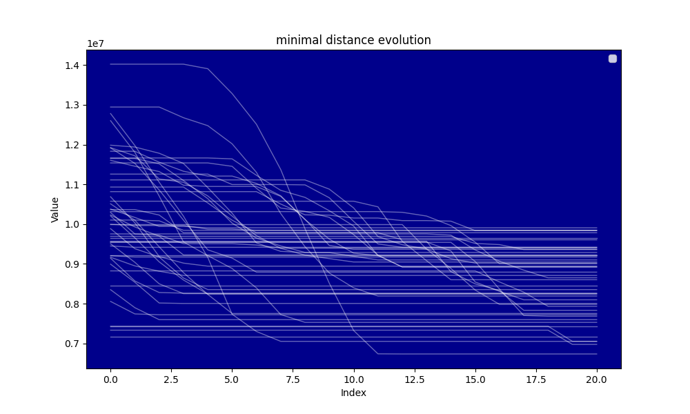
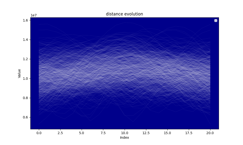
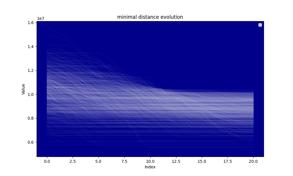
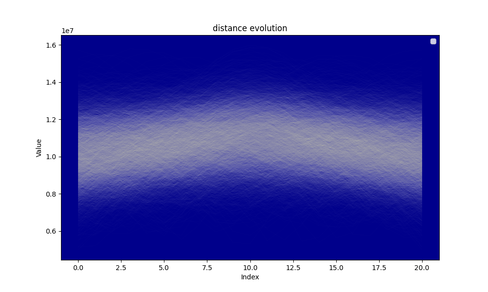
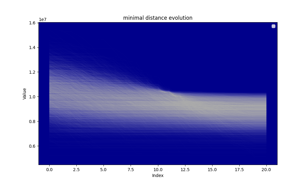
The analysis shows that for and the average distance at the beginning of the circular mean centering is approximately and the average distance at the end of the circular mean centering is , thus the distance reduction is which is approximately . The distance reduction is thus close to
Our model is thus not very good, the average distance reduction by step is and the simulation seems to show that on average the search tends to increase the distance at mid procedure rather than reducing it, yet a clear reduction of the distance is observed. A potential explanation is the skewness of the distribution of the distances at the beginning of the circular mean centering procedure. The smallest distances tend to be further from the mean than the greatest distances.
implementation
Hereafter is a first simple version of the algorithm that works for small keys, knowing only the total hamming weight of the key.
For 2000000 samples, with a noise having a standard deviation of 50 and a threshold of which means samples are selected if , you should get a result looking like that:
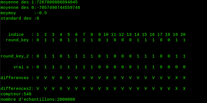
V is for a match between the real key and the key found, and X is for a mismatch. Lowering the threshold gives better results, but you need more samples.
use rand::Rng;
use rand::rng;
use rand_distr::{Uniform, Normal, Distribution};
use rayon::prelude::*;
use std::convert::TryInto;

fn roll_subarray<const K: usize, const K_1: usize>(array: &mut [i64; K_1], start: usize, end: usize) -> i64 {
    let m = end - start;
    assert!(m <= K, "m must be less than or equal to K");

    let mut temp_array: Vec<i128> = array[start..end].iter().map(|&x| x as i128).collect();
    let mut best_distance = i128::MAX;
    let mut best_array = temp_array.clone();
    let mut final_mean = 0;

    for _ in 0..m {
        let mean: i128 = temp_array.iter().sum::<i128>() / (m as i128);
        let distance: i128 = temp_array.iter().fold(0, |acc, &x| acc + (x - mean).abs());

        if distance < best_distance {
            //println!("distance:{}",(distance as f64).log2());
            best_distance = distance;
            best_array.copy_from_slice(&temp_array);
            final_mean = mean;
        }

        if let Some((index, _)) = temp_array.iter().enumerate().min_by_key(|&(_, &x)| x) {
            temp_array[index] += 1i128 << 64;
        }
    }

    let mod_mask = (1i128 << 64) - 1;

    array[start..end].iter_mut().zip(best_array.iter())
        .for_each(|(a, &v)| *a = ((v - final_mean) & mod_mask) as i64);

    (final_mean & mod_mask) as i64
}


//main single hamming weight
//*
fn main() {
    // Taille du vecteur et des tableaux
    let n: usize = 4_000_000; // Taille de l'échantillon
    const K: usize = 20; // dimension du vecteur lwe
    const K_1: usize = 21;
    let hamming = 10; // Nombre de valeurs non nulles dans s
    let threshold = 65.3;

    // Distribution uniforme pour les valeurs a[i]
    let uniform_dist = Uniform::new(i64::MIN, i64::MAX).expect("Failed to create uniform distribution");

    // Distribution gaussienne pour l'erreur e
    let sigma = 50.0;
    let normal_dist = Normal::new(0.0, sigma).expect("Failed to create normal distribution");


    // Générer le tableau s de taille K avec un nombre spécifié de valeurs non nulles
    let mut s = vec![0; K];
    let mut t = 0;
    while t < hamming {
        let index = (rng().random::<u64>() % (K as u64)) as usize;
        if s[index] == 0
        {
            s[index] = 1;
            t+= 1;
        }

    }


    let mut vect: Vec<[i64; K + 1]> = (0..n)
        .into_par_iter() // Utilisation de rayon pour paralléliser
        .map(|_| {
            // Créer un générateur de nombres aléatoires pour chaque thread
            let mut rng = rand::rng();
            let mut array: [i64; K + 1] = [0; K + 1];

            // Générer les K premières valeurs a[i]
            for i in 0..K {
                array[i] = uniform_dist.sample(&mut rng);
            }


            // Calculer la somme pondérée avec une erreur gaussienne
            let sum: i64 = s.iter().zip(&array[..K]).map(|(&si, &ai)| si * ai).sum();
            let error: i64 = normal_dist.sample(&mut rng) as i64;
            let last_value = sum + error;

            // Ajouter la valeur calculée au tableau
            array[K] = last_value;

            array
        })
        .collect();

    // Moyenne circulaire
    //*
    vect.par_iter_mut().for_each(|x|{
        let mean = roll_subarray::<K,K_1>( x, 0, K);
        x[K] = x[K] - (((mean as i128)*(hamming as i128)) as i64);
    });
    // */

        // Fonction pour sélectionner les tableaux en parallèle


    let mut selected_vect: Vec<[i64; K + 1]> = vect.into_par_iter()
        .filter(|&array|{
            let acc = array[..K].iter().map(|&x| x.abs() as i128).sum::<i128>() as i128;
            (acc as f64).log2() < threshold
        })
        .collect();


    let mut b:Vec<i128> =vec![0;K];
    let mut moyenne_a = vec![0i128;K];

    let len = selected_vect.len();
    for j in 0..len
    {
        moyenne_a.iter_mut().zip(selected_vect[j].iter()).for_each(|(x,y)|{ *x= *x + (*y).abs() as i128 } );
        b.iter_mut().zip(selected_vect[j].iter()).for_each(|(x,y)|{*x= *x +(((*y).signum())*selected_vect[j][K]) as i128 } );
    }
    println!();


    let mut max=moyenne_a[0];
    moyenne_a.iter_mut().for_each(|x|{if *x > max{max = *x};});
    let moy_b:i128 = (b.iter().sum::<i128>())/(K as i128);
    b.iter_mut().for_each(|x|{*x = *x -moy_b ;println!("b {}",*x)});

    b.iter_mut().zip(moyenne_a.iter_mut()).for_each(|(x,y)|{
        if *y != 0
        {
            let temp= (*x)*((max)/(*y));
            if (*x) > 0 && temp < 0 || (*x) < 0 && temp > 0
            {
                println!("parité{}",*x);
            }
            *x = ((*x as f64)*((max as f64)/(*y as f64))) as i128;
        }
    });

    let mut r:Vec<f64> = vec![0.0;K];

    println!();
    println!(" faux s: ");

    for i in 0..K
    {
        r[i]= (b[i] as f64)/((K*len) as f64) ;  //-0.5;
        println!(" {} :{} ",i+1,r[i]);
    }

    let mut moy0:f64 =0.0;
    let mut moy1:f64 =0.0;
    let mut standard_dev=0.0;
    let mut compt0:f64 =0.0;
    let mut compt1:f64 =0.0;
    for i in 0..K{
        if s[i] == 1 {
            moy1+=r[i];
            compt1+=1.0;
        }else{
            moy0+=r[i];
            compt0+=1.0;
        }
    }

    standard_dev = standard_dev/(K as f64-1.0);
    standard_dev = standard_dev.sqrt();
    let moymoy =-0.5;
    moy0=moy0/compt0;
    moy1=moy1/compt1;
    println!("moyenne des 1:{}",moy1);
    println!("moyenne des 0:{}",moy0);
    println!("moymoy       :{}",moymoy);
    println!("standard dev :{}",standard_dev);
    println!();
    let mut round_key:Vec<i64> = vec![0;K];
    let mut round_key_2:Vec<i64> = vec![0;K];
        for i in 0..K{
            if r[i] < 0.0{
                round_key[i]=0;
            }
            else{
                round_key[i]=r[i].round() as i64;
            }
            if round_key[i] > 1{
                round_key[i]=1;
            }
        }
        for i in 0..K{
            if r[i]-moymoy < 0.0{
                round_key_2[i]=0;
            }
            else{
                round_key_2[i]=(r[i]-moymoy).round() as i64;
            }
            if round_key_2[i] > 1{
                round_key_2[i]=1;
            }
        }

    println!();
    print!("   indice   :");
    for i in 0..K{
        if i+1<10{
            print!(" {} ",i+1);
        }else{
            print!("{} ",i+1);
        }

    }
    println!();
    print!("  round_key :");
    for i in 0..K{
        print!(" {} ",round_key[i]);
    }
    println!();
    println!();
    println!();
    print!("round_key_2 :");
    for i in 0..K{
        print!(" {} ",round_key_2[i]);
    }
    println!();
    println!();

    print!("     vrai s :");
    for i in 0..K{
        print!(" {} ",s[i]);
    }

    println!();
    println!();

    print!("differences :");
    for i in 0..K{
        if round_key[i]-(s[i] as i64)==0{
           print!(" V ");
        }else{
           print!(" X ");
        }
    }
    println!();
    println!();

    print!("differences2:");
    for i in 0..K{
        if round_key_2[i]-(s[i] as i64)==0{
           print!(" V ");
        }else{
           print!(" X ");
        }
    }
    println!();
    println!("compteur:{}",len);
    println!("nombre d'echantillons:{}",n);

}

// */
Instead of assuming we know the hamming weight of the key, we now assume we know the hamming weights of chunks of arbitrary size the key. In a real life situation, instead of assuming we know them, we can just try all the possible hamming weigts of each chunk. For example, if the key is of sie 60, and we have 3 chunks of eual size, then the chunks have a size of 20, then the key can have either 0,1,2 or ...20 non zero bits. Thus in a real life situation, we can just try all the possible hamming weights, and apply the same algorithm. That brute force method would multiply the duration of the calculation by , although, it’s still unlikely that 20 bits in a row would all be 0 or 1.
In practice though, the bigger the chunk is, the smaller is the relative standard deviation of the number of non zero bits in that chunk. i.e. For a 100 bits key chunk, the average hamming weight is , with a . With a confidence, the hamming weight of the chunk is thus between and .
If the chunk has a size of 20 bits, you can expect that approximately 60% of the hamming weights to be between 7.77 and 12.23, and 95% of them to be between 5.54 and 14.46. So in most cases, the brute force method would likely end before trying different hamming weights.
Dividing the key in chunks of aritrary size allows the number of valid samples to increase by a lot.
In the code, the function that finds the circular mean is called "roll_subarray". We apply the "roll_subarray" function to chunks of size 20 for each sample. The function is linear in with n the sie of the key, so for m samples, that’s . Some parallelism might reduce that but each key chunk is too small to suffer the overhead provoked by parallelism.
The roll_subarray function finds the circular mean of each chunk and center all the sample values around that mean.
The function allows to slightly transform the distribution, then, we can make linear combinations between transformed samples to increase the likelihood of finding "small" samples little by little.
We start with 40 000 samples, and a threshold of . We recovered 55 bits of the key, to recover 60 bits, the algo needs to start with more samples and or have a lower threshold. Let’s go higher.

Twin samples
As explained previously, the data treatment needs to have samples whose components are "small" to recover the key.
By using the hamming weight, we can also recover a key using samples whose components are "close" to their mean, i.e. samples which have only small variations.
The probability of picking up two samples having close components up to a range is
The probability of not picking up two samples having close components up to a range is
In a set of m samples, the probability of having no pair of samples having close components up to a range is
So the probability of finding at least one pair is
and the average number of pairs is equal to the average number of collisions
sample with small variations between components
We can increase furthermore the number of acceptable samples by using linear combinations between samples. By making linear combinations of samples which only have close variations, (neither small nor having small components), and using the hamming weight, we can get more samples. We call them twin samples. Twin samples are samples whose components have approximately the same variations. For example, with the modulus and representatives in and two samples, and , . The variations between the first 4 components are rather small, (1,1,-1), so we call them twin samples. By knowing the hamming weight, we can change it to by removing to each component and modifying the last components .
The new algorithm is described at high level here:
The idea is to first reduce the distance of the first chunk by linear combination until it becomes very small. Since we do not look at the other components, they keep being distributed with a uniform distribution.
Then, the same method is applied to the first two chunks, then to the first three chunks etc...
The new version of the program should use a Cargo.toml file looking like that:
[package]
name = "attack_find"
version = "0.1.0"
edition = "2021"

[dependencies]
rand = "0.9.1"
rand_distr = "0.5.1"
rayon = "1.10.0"
tikv-jemallocator = "0.6"

[profile.release]
codegen-units = 1
lto = "fat"
and to run it, I suggest using the command:
RUSTFLAGS="-C target-cpu=native" cargo build --release// */
#[global_allocator]
static GLOBAL: tikv_jemallocator::Jemalloc = tikv_jemallocator::Jemalloc;
use rand::Rng;
use rand::rng;
use rand_distr::{Uniform, Normal, Distribution};
use rayon::prelude::*;
use std::sync::atomic::{AtomicUsize, Ordering};
#[inline(always)]
fn find_a_twin_sub<const K: usize, const K_1: usize>(
array_1: &mut [i64; K_1],
array_2: &mut [i64; K_1],
hi: usize,
start: usize,
end: usize
) -> i128 {
let mut temp_array_1 = *array_1;
let temp_array_2 = *array_2;
let mut best_distance: i128 = temp_array_1[start..end].iter().fold(0, |acc, &x| acc + x.abs() as i128);
temp_array_1.iter_mut().zip(temp_array_2.iter()).for_each(|(x, y)| *x -= *y);
let mean = roll_subarray::<K, K_1>(&mut temp_array_1, start, end);
temp_array_1[K] -= mean * (hi as i64);
let distance: i128 = temp_array_1[start..end].iter().fold(0, |acc, &x| acc + x.abs() as i128);
if distance < best_distance {
best_distance = distance;
*array_1 = temp_array_1;
}
best_distance
}
#[inline(always)]
fn find_a_twin_add<const K: usize, const K_1: usize>(
array_1: &mut [i64; K_1],
array_2: &mut [i64; K_1],
hi: usize,
start: usize,
end: usize
) -> i128 {
let mut temp_array_1 = *array_1;
let temp_array_2 = *array_2;
let mut best_distance: i128 = temp_array_1[start..end].iter().fold(0, |acc, &x| acc + x.abs() as i128);
temp_array_1.iter_mut().zip(temp_array_2.iter()).for_each(|(x, y)| *x += *y);
let mean = roll_subarray::<K, K_1>(&mut temp_array_1, start, end);
temp_array_1[K] -= mean * (hi as i64);
let distance: i128 = temp_array_1[start..end].iter().fold(0, |acc, &x| acc + x.abs() as i128);
if distance < best_distance {
best_distance = distance;
*array_1 = temp_array_1;
}
best_distance
}
//*
fn reduce_by_twin<const K: usize, const K_1: usize>(
vec_1: &mut Vec<[i64; K_1]>,
vec_2: &mut Vec<[i64; K_1]>,
n: usize,
h_v: &[usize],
nb_chunck: usize
) {
let h_vec = h_v.to_vec();
let h_len = h_vec.len();
let len = vec_1.len();
let l = vec_2.len();
let num_threads = rayon::current_num_threads();
let progress = AtomicUsize::new(0);
for k in 0..h_len {
let f = (k + 1) * K / nb_chunck;
let ini = k * K / nb_chunck;
for r in 1..(n + 1) {
let chunck_size = (len + num_threads - 1) / num_threads;
let chunks: Vec<(usize, usize)> = (0..num_threads)
.map(|i| (i * chunck_size, (i + 1).min(len / chunck_size + 1) * chunck_size))
.collect();
let results: Vec<Vec<[i64; K_1]>> = chunks.into_par_iter().map(|(start, end)| {
let mut local_vec_1 = vec_1[start..end.min(len)].to_vec();
let mut local_vec_2 = vec_2.clone();
let mut vec_sub = local_vec_1.clone();
let mut vec_add = local_vec_1.clone();
let vec_ta = local_vec_1.clone();
for i in 0..local_vec_1.len() {
let mut vec_temp_sub = vec_sub[i];
let mut vec_temp_add = vec_add[i];
let vec_tamp = vec_ta[i];
let mut bd = local_vec_1[i][ini..f].iter().fold(0, |acc, &x| acc + x.abs() as i128);
for j in (start + i + 1)..l {
let ds = find_a_twin_sub::<K, K_1>(&mut vec_temp_sub, &mut local_vec_2[j], h_vec[k], ini, f);
let da = find_a_twin_add::<K, K_1>(&mut vec_temp_add, &mut local_vec_2[j], h_vec[k], ini, f);
if ds < bd && ds < da {
let bd_2 = local_vec_1[i][0..ini].iter().fold(0, |acc, &x| acc + x.abs() as i128);
let ds_2 = vec_temp_sub[0..ini].iter().fold(0, |acc, &x| acc + x.abs() as i128);
if ds_2 <= bd_2
{
bd = ds;
local_vec_1[i].copy_from_slice(&vec_temp_sub);
}
} else if da < bd {
let bd_2 = local_vec_1[i][0..ini].iter().fold(0, |acc, &x| acc + x.abs() as i128);
let da_2 = vec_temp_add[0..ini].iter().fold(0, |acc, &x| acc + x.abs() as i128);
if da_2 <= bd_2
{
bd = da;
local_vec_1[i].copy_from_slice(&vec_temp_add);
}
}
vec_temp_sub.copy_from_slice(&vec_tamp);
vec_temp_add.copy_from_slice(&vec_tamp);
}
//let progress_val = progress.fetch_add(1, Ordering::SeqCst);
//if progress_val % 10 == 0 {
println!("bd:{} r:{} i:{} k:{}", (bd as f64).log2(), r, i, k);
//}
}
local_vec_1
}).collect();
vec_1.par_chunks_mut(chunck_size)
.zip(results)
.for_each(|(chunk, result)| {
chunk.copy_from_slice(&result[..chunk.len()]);
});
vec_2.copy_from_slice(vec_1);
}
}
}
// */
#[inline(always)]
fn roll_subarray<const K: usize, const K_1: usize>(array: &mut [i64; K_1], start: usize, end: usize) -> i64 {
let m = end - start;
assert!(m <= K, "m must be less than or equal to K");
let mut temp_array: Vec<i128> = array[start..end].iter().map(|&x| x as i128).collect();
let mut best_distance = i128::MAX;
let mut best_array = temp_array.clone();
let mut final_mean = 0;
for _ in 0..m {
let mean: i128 = temp_array.iter().sum::<i128>() / (m as i128);
let distance: i128 = temp_array.iter().fold(0, |acc, &x| acc + (x - mean).abs());
if distance < best_distance {
best_distance = distance;
best_array.copy_from_slice(&temp_array);
final_mean = mean;
}
if let Some((index, _)) = temp_array.iter().enumerate().min_by_key(|&(_, &x)| x) {
temp_array[index] += 1i128 << 64;
}
}
let mod_mask = (1i128 << 64) - 1;
array[start..end].iter_mut().zip(best_array.iter())
.for_each(|(a, &v)| *a = ((v - final_mean) & mod_mask) as i64);
(final_mean & mod_mask) as i64
}
fn reduce_hamming_weight<const K: usize, const K_1: usize>(
sample: &mut [i64; K_1],
h_v: &[usize],
)
{
let n = h_v.len();
let size = K/n;
for i in 0..n
{
if h_v[i] > (size>>1)
{
let sum = sample[i*size..(i+1)*size].iter().sum::<i64>();
sample[K] -= sum;
}
}
}
fn main() {
let n: usize = 40000;
const K: usize = 60;
const K_1: usize = 61;
let threshold = 65.65;
let n_chunck = 3;
let cs= K/n_chunck;
const NC: usize = 3;
let mut h_vec = [0; NC];
let h: usize = 30;
let n_round = 10;
let uniform_dist = Uniform::new(i64::MIN, i64::MAX).expect("Failed to create uniform distribution");
let sigma = 10.0;
let normal_dist = Normal::new(0.0, sigma).expect("Failed to create normal distribution");
let mut s = vec![0; K];
let mut t = 0;
while t < h
{
let index = (rng().random::<u64>() % (K as u64)) as usize;
if s[index ] == 0
{
s[index ] = 1;
t += 1;
}
}
for i in 0..n_chunck
{
h_vec[i] = (s[i*cs..(i+1)*cs].iter().sum::<i64>()) as usize;
}
let mut vect: Vec<[i64; K + 1]> = (0..n)
.into_par_iter()
.map(|_| {
let mut rng = rand::rng();
let mut array: [i64; K + 1] = [0; K + 1];
for i in 0..K {
array[i] = uniform_dist.sample(&mut rng);
}
let sum: i64 = s.iter().zip(&array[..K]).map(|(&si, &ai)| si * ai).sum();
let error: i64 = normal_dist.sample(&mut rng) as i64;
let last_value = sum + error;
array[K] = last_value;
array
})
.collect();
let mut vect_2 = vect.clone();
reduce_by_twin::<K, K_1>(&mut vect, &mut vect_2, n_round, &h_vec, n_chunck);
for mut s in &mut vect
{
reduce_hamming_weight::<K,K_1>(&mut s, &h_vec);
}
let selected_vect: Vec<[i64; K + 1]> = vect.clone().into_par_iter()
.filter(|&array| {
let acc = array[..K].iter().map(|&x| x.abs() as i128).sum::<i128>() as i128;
(acc as f64).log2() <= threshold
})
.collect();
let mut b: Vec<i128> = vec![0; K];
let mut moyenne_a = vec![0i128; K];
let len = selected_vect.len();
for j in 0..len {
moyenne_a.iter_mut().zip(selected_vect[j].iter()).for_each(|(x, y)| { *x = *x + (*y).abs() as i128 });
b.iter_mut().zip(selected_vect[j].iter()).for_each(|(x, y)| { *x = *x + ((*y).signum() * selected_vect[j][K]) as i128 });
}
let mut max = moyenne_a[0];
moyenne_a.iter_mut().for_each(|x| { if *x > max { max = *x } });
let moy_b: i128 = (b.iter().sum::<i128>()) / (K as i128);
b.iter_mut().for_each(|x| { *x = *x - moy_b });
b.iter_mut().zip(moyenne_a.iter_mut()).for_each(|(x, y)| {
if *y != 0 {
*x = ((*x as f64) * ((max as f64) / (*y as f64))) as i128;
}
});
let mut r: Vec<f64> = vec![0.0; K];
for i in 0..K {
r[i] = (b[i] as f64) / ((K * len) as f64);
}
let mut moy0: f64 = 0.0;
let mut moy1: f64 = 0.0;
let mut compt0: f64 = 0.0;
let mut compt1: f64 = 0.0;
for i in 0..K {
if s[i] == 1 {
moy1 += r[i];
compt1 += 1.0;
} else {
moy0 += r[i];
compt0 += 1.0;
}
}
moy0 = moy0 / compt0;
moy1 = moy1 / compt1;
println!("moyenne des 1: {}", moy1);
println!("moyenne des 0: {}", moy0);
println!("compteur: {}", len);
println!("nombre d'echantillons: {}", n);
let mut round_key: Vec<i64> = vec![0; K];
let mut round_key_2: Vec<i64> = vec![0; K];
for i in 0..K {
if r[i] < 0.0 {
round_key[i] = 0;
} else {
round_key[i] = r[i].round() as i64;
}
if round_key[i] > 1 {
round_key[i] = 1;
}
}
for i in 0..K {
if r[i] - (-0.5) < 0.0 {
round_key_2[i] = 0;
} else {
round_key_2[i] = (r[i] - (-0.5)).round() as i64;
}
if round_key_2[i] > 1 {
round_key_2[i] = 1;
}
}
println!(" indice :");
for i in 0..K {
print!(" {}", i + 1);
}
println!();
println!(" round_key :");
for i in 0..K {
print!(" {}", round_key[i]);
}
println!();
println!("round_key_2 :");
for i in 0..K {
print!(" {}", round_key_2[i]);
}
println!();
println!(" vrai s :");
for i in 0..K {
print!(" {}", s[i]);
}
println!();
println!("differences :");
for i in 0..K {
if round_key[i] - (s[i] as i64) == 0 {
print!(" V ");
} else {
print!(" X ");
}
}
println!();
println!("differences2:");
for i in 0..K {
if round_key_2[i] - (s[i] as i64) == 0 {
print!(" V ");
} else {
print!(" X ");
}
}
println!();
println!("compteur: {}", len);
println!("nombre d'echantillons: {}", n);
}